library(tidyverse)BIOL 5404 Assignment 2
Instructions
- Create a new .R script to complete this assignment in your local assignments folder for this course.
- You’ll submit the .R script on Brightspace.
- Put your FIRST and LAST NAME in the file name of the script.
- Put your name at the top of the script as well.
- Please do not include your student ID, just your name is enough.
- Show your work!
- Make sure your script is organized and legible.
- Use code sections (####) & question numbers as outlined below.
- Provide all written answers as brief # comments within your script.
- Be sure to load all packages needed at the top of your script, like this (adding any other packages needed):
We will use the diamonds dataset that comes with the tidyverse package. We will also use the iris dataset that comes with base R.
Part 1
In R, the sd() function takes a vector of numeric data and returns the sample standard deviation.
x <- 1:10
sd(x)
[1] 3.027651a. Write your OWN function that takes a vector of numeric data, and returns the sample standard deviation (you’ll need to know the formula for SD to do this).
Use the formula for the Sample SD here:
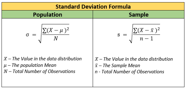
Note: do not use sd() in your function! The purpose of this exercise is to generate a function yourself that will do this.
1b. Verify that your function gives the same output as sd() for a few examples. What happens if you pass your function a vector of character data? What happens if you pass your function a vector that is a factor?
1c. Now, modify your function so that IF it gets passed a vector that is not numeric, THEN it prints a useful error message. Start by copy-pasting your function above, then modify it to add this new capacity. After creating your new-and-improved function, show that it works with a few examples.
Hint: you can use a conditional statement to do this, along with the function is.numeric(), which is shown below.
is.numeric(1:10)[1] TRUEis.numeric(c('a', 'b', 'c'))[1] FALSE1d. What happens if you pass your function a numeric vector that has one NA value in it?
OPTIONAL: Modify your function further (building a new version) so that if it gets passed a numeric vector with at least one NA entry, it still reports the sample SD for the non-NA values. How many non-NA datapoints (values) does your function need, at a minimum, to be able to report the SD? Caution: ensure that your function calculates the sample sd of non-NA values using the correct n of non-NA values.
Part 2
2a. Building on the function you created above, write a new function (with a new name) that takes a vector of values as input, and calculates and returns 3 descriptive statistics:
- the sample mean,
- the sample SD,
- and the standard error of the mean.
It should return a vector of those three values.
2b. To maximize the usefulness of this new function, modify it so that the 3 values in the vector that gets returned are each named. Here is a hint/reminder for how to create a vector of numeric values where each element has a name:
c('mean' = 1, 'sd' = 2, 'sem' = 3)mean sd sem
1 2 3 Part 3
3a. Write a for loop that prints the values from 50:80
3b. The iris dataset has measurements of flower morphology for 3 iris species:
str(iris)'data.frame': 150 obs. of 5 variables:
$ Sepal.Length: num 5.1 4.9 4.7 4.6 5 5.4 4.6 5 4.4 4.9 ...
$ Sepal.Width : num 3.5 3 3.2 3.1 3.6 3.9 3.4 3.4 2.9 3.1 ...
$ Petal.Length: num 1.4 1.4 1.3 1.5 1.4 1.7 1.4 1.5 1.4 1.5 ...
$ Petal.Width : num 0.2 0.2 0.2 0.2 0.2 0.4 0.3 0.2 0.2 0.1 ...
$ Species : Factor w/ 3 levels "setosa","versicolor",..: 1 1 1 1 1 1 1 1 1 1 ...The first 4 columns are numeric measurements of length and width of flower structures. Write a for loop that:
- Generates a histogram for each of those 4 columns in turn.
- Each histogram should have a title on top of the histogram with the name of the column (Petal.Width, etc).
- Hint: you can do this with hist() using the main argument in base R
- Other hint: column names for a data.frame are accessible via names()
- And lastly, your loop should wait for a keypress before moving on to the next column and generating the next histogram.
- Hint: one way to pause to wait for a keypress in the console is to use the readline() function:
readline(prompt = 'Press return/enter to continue')Part 4
4a. Use apply() to get the median value for each of the first 4 columns of the iris dataset.
4b. Create an 8 x 8 matrix (give it a name) with the values from 1:64, where the values are filled in row-wise (i.e., the first row should be 1:8, second should be 9:16, third should be 17:24, etc)
4c. Use apply() to get the sample sd of each column in your matrix.
4d. Use apply() to get the sample sd of each row in your matrix. Are you surprised by the values?
Part 5
For this question, we’ll use the diamonds dataset. It is a large dataset with data on the characteristics from ~54,000 diamonds, including each diamond’s weight in carats; it’s “cut”, color, and clarity classifications; it’s price; and it’s dimensions (mm) in 3 axes (and a few others variables).
diamonds# A tibble: 53,940 × 10
carat cut color clarity depth table price x y z
<dbl> <ord> <ord> <ord> <dbl> <dbl> <int> <dbl> <dbl> <dbl>
1 0.23 Ideal E SI2 61.5 55 326 3.95 3.98 2.43
2 0.21 Premium E SI1 59.8 61 326 3.89 3.84 2.31
3 0.23 Good E VS1 56.9 65 327 4.05 4.07 2.31
4 0.29 Premium I VS2 62.4 58 334 4.2 4.23 2.63
5 0.31 Good J SI2 63.3 58 335 4.34 4.35 2.75
6 0.24 Very Good J VVS2 62.8 57 336 3.94 3.96 2.48
7 0.24 Very Good I VVS1 62.3 57 336 3.95 3.98 2.47
8 0.26 Very Good H SI1 61.9 55 337 4.07 4.11 2.53
9 0.22 Fair E VS2 65.1 61 337 3.87 3.78 2.49
10 0.23 Very Good H VS1 59.4 61 338 4 4.05 2.39
# ℹ 53,930 more rows
Remember, you can use this to see the meta-data:
help(diamonds)5a. What are the possible values of cut? Take a look at them, and examine the distribution of cut (i.e., the number of diamonds in the dataset in each cut category).
5b. Suppose we want to model the relationship between price and weight (carat) for each cut separately (in a separate model). As a first step, create a scatterplot for price vs. carat weight for JUST the subset of Premium diamonds from the dataset. You can use ggplot2 if you wish, or just use plot() in base R.
5c. Now, regenerate the scatterplot, but this time plot natural log-transformed price vs. natural log-transformed carat weight, for just the Premium diamonds. How does the relationship change when examining the log-log transformation?
5d. Create an object mod that is a fitted regression model for log-price vs. log-carat weight for just the Premium diamonds. Examine the summary() for your model. What % of variation in the log-price of premium diamonds is explained by log-weight? (This is the multiple R-squared.)
5e. Show that you can extract the value of this R-squared from the fitted model.
Hint: summary(mod) is itself a list object that contains the value you are looking for. You can use str() on the output of summary(mod) to determine the names of elements within summary(mod). Then use the appropriate name to index (i.e., pull out) the R-squared value.
OPTIONAL: Write a custom function that takes a fitted model object, and returns the R-squared value from its summary.
Extra optional challenges
This is for extra (excellent) practice, and is not graded.
Use a for loop to fit a separate model of log-price vs. log-weight for EACH of the levels of cut in the diamonds dataset (Ideal, Premium, Good etc), and store the fitted model in a list.
To get you started, the example below creates an empty list called fitted_mods with a length that matches the number of unique levels of cut (5). Write your for loop so that it iterates over each level of cut, fitting the log-log regression model (as you did above), and then storing the fitted model in the appropriate slot of fitted_mods. When your loop is done, fitted_mods should contain one fitted model for each unique cut type.
mycuts <- unique(diamonds$cut)

fitted_mods <- vector("list", length = length(mycuts))
Using sapply() and your function for extracting R-squared values, get the five R-squared values from your fitted_mods list.
Looking at the meta-data for diamonds, we see that the column depth is a measure of diamond shape that is calculated from a diamond’s linear x, y, and z dimensions. The help file gives two separate formulas for depth, as follows:
z / mean(x, y)
2 * z / (x + y)
…and somewhat confusingly, after the formulas, it also gives the range of depth values in the dataset, reported as (43-79). We can confirm this with:
summary(diamonds$depth)Min. 1st Qu. Median Mean 3rd Qu. Max. 43.00 61.00 61.80 61.75 62.50 79.00Create a new column in diamonds, depthF2, that calculates depth following the second formula above.
Create a new column in diamonds, depthF1, that calculates depth following the first formula above.
Plot a scatterplot of depthF1 vs. depthF2. Add a red line that shows a 1:1 relationship. Note that there are many ways to do this, and one is abline(). Does the result look as you would expect?
Looking at the range of your newly calculated values, it’s clear that the depth column in diamonds is scaled by some factor. Can you figure out what that factor is, using the data?
Re-scale your newly-calculated columns depthF2 and depthF1 so that they are expected to match depth. Then plot depth vs. one of your new columns. Add the red 1:1 line again.
It’s clear from the plot that the dataset has some discrepancies. Either we have errors in the x, y, or z measurements, OR we have errors in the depth values that were calculated by the authors of the diamonds dataset (or both). Investigating this, which do you think is more likely?
Let’s create a marker to identify the problematic rows. Generate a new column in diamonds called meas_ok that has a value of T IF the measurements are OK, and a value of F if there is a large discrepancy that we would want to investigate futher.
As the definition of a “large enough” discrepancy for this example, let’s say if your calculated depthF1 is within +/- 5 of the value in depth column of the dataset, we’ll consider that row to be OK.
IF depthF1 and depth have a discrepancy that is larger than +/- 5, or if depthF1 is missing or NA, consider it to be a problematic row.
How many of the diamonds are problematic? What percent of the original data is this? Create a filtered data.frame with just the problematic rows, so they can be inspected.