library(tidyverse)
library(rmarkdown)Billboard top 100 from Y2K

What was pop music like then?
The billboard data that comes with tidyverse in R includes rankings for popular songs from the Billboard “Top 100” weekly chart from the year 2000. Let’s explore these data. Some questions we will investigate include:
At the song level,
- What is a typical song’s tenure on the charts?
- Is there a relationship between a song’s tenure and its peak rank?
At the artist level,
- Which artists have multiple hits?
- Is there variation in popularity (song rank) even within the upper-echelon of pop stars?
At the chart level,
- How does turnover change throughout the year?
- Does the number of fresh songs on the chart change with season?
- Do some seasons have greater fluctuations in song rank than others?
We’ll start by loading the tidyverse and rmarkdown packages.
The billboard dataset comes in wide format initially, with one row per song:
paged_table(billboard[1:20,])Reshape the data
We’ll set up a tidy dataframe, with one row per song-rank, and remove the NAs (where there is no rank for a given song). We will also calculate the date for each song-rank, based on the song’s entry date plus the number of weeks it had been on the chart, according to the data:
Code
dat <- billboard %>% pivot_longer(cols = 4:79, names_to = 'week', values_to = 'rank') %>%
  mutate(year_entered = year(date.entered)) %>%
  mutate(week_num = as.numeric(substr(week, 3, nchar(week)))) %>%
  mutate(date_rank = date.entered + (7 * (week_num - 1))) %>%
filter(!is.na(rank))paged_table(dat)So, we have 317 tracks by 228 artists. Somehow, Y2K had two charting tracks with the same name!
Reality checks (hygiene)
Let’s get a handle on some basic checks.
# A tibble: 2 × 2
  year_entered     n
         <dbl> <int>
1         1999    50
2         2000   267
Some of the songs in this dataset entered the ranks in the year 1999.
Check the rank values to make sure they’re as expected:
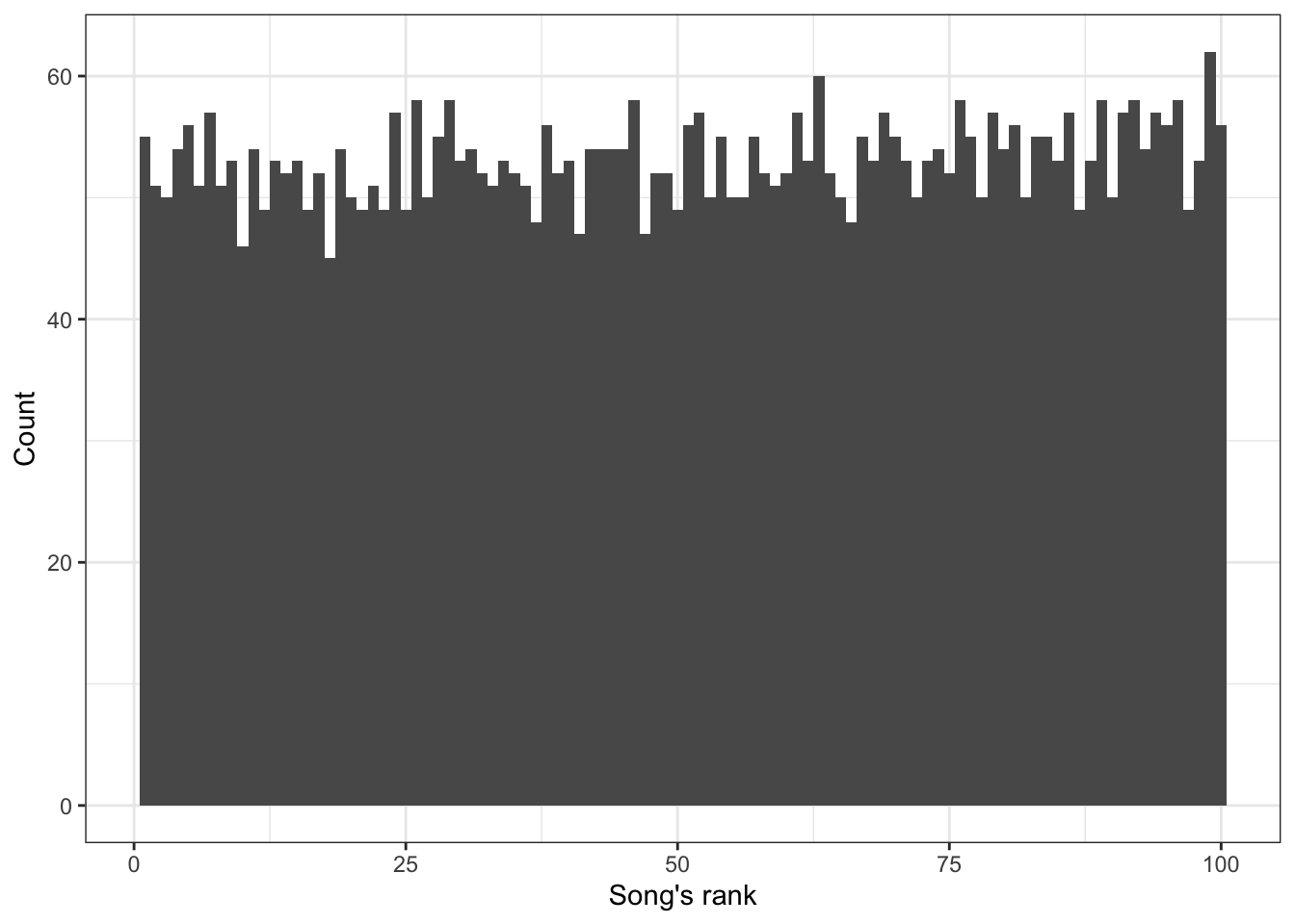
As expected, the ranks range from 1 to 100.
Let’s check that the specific dates of each rank correspond to a set of discrete weekly dates, as expected for the Billboard releases (i.e., we should have a limited set of dates that correspond to a weekly release of the billboard list):
dat %>% ggplot() + theme_bw() +
  geom_bar(aes(x = date_rank), width = 0.9) + labs(y = 'Count', x = 'Date')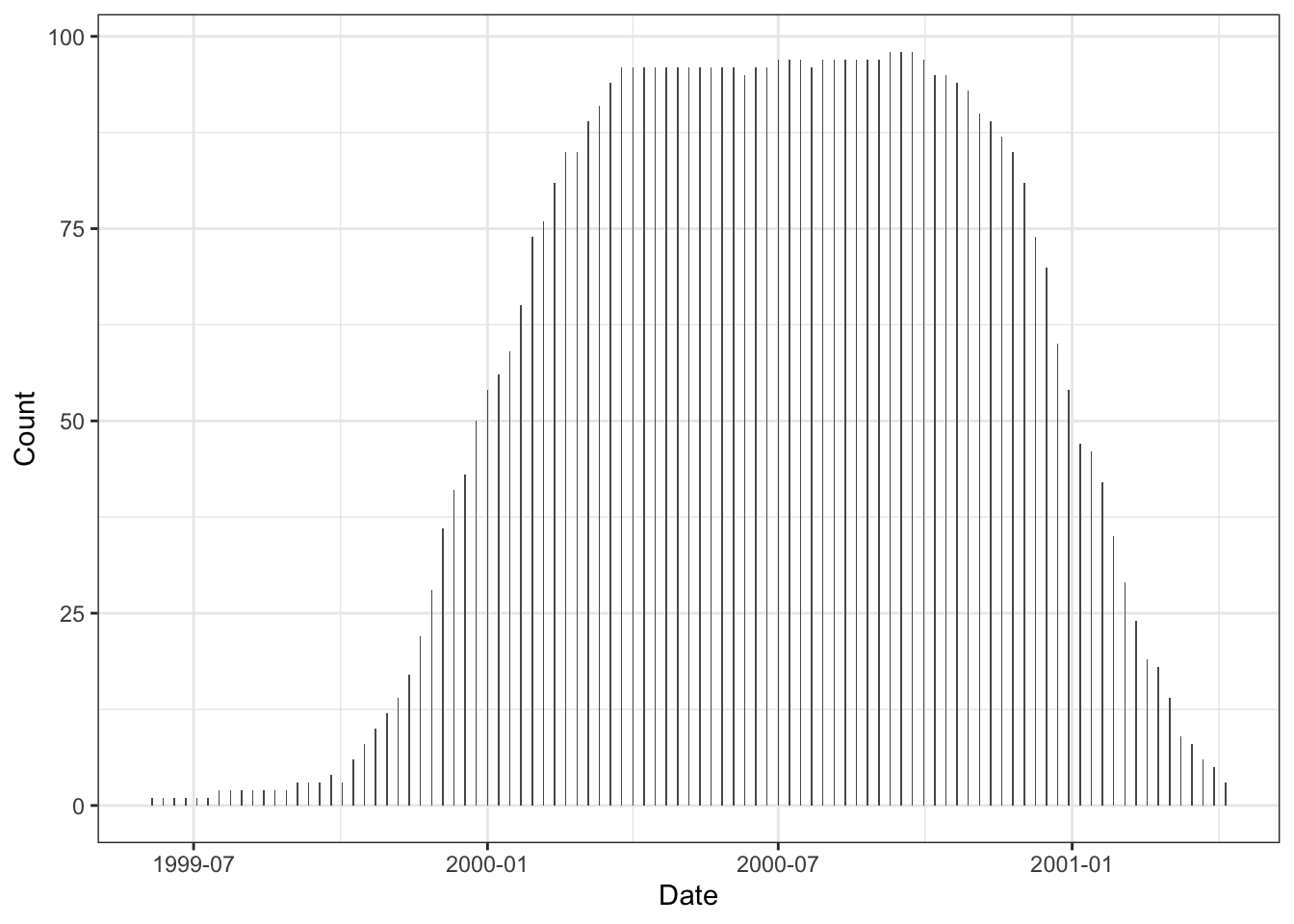
release_dates <- dat %>%
  filter(!duplicated(date_rank)) %>%
  select(date_rank) %>%
  arrange(date_rank) %>%
  mutate(interval = date_rank - lag(date_rank))

release_dates %>%
  filter(!is.na(interval)) %>%
  group_by(interval) %>%
  tally() # all 7 days apart, as expected
# A tibble: 1 × 2
interval n
<drtn> <int>
1 7 days 96release_dates %>%
mutate(d_of_week = wday(date_rank, label = T)) %>% # lubridate
group_by(d_of_week) %>% tally()# A tibble: 1 × 2
d_of_week n
<ord> <int>
1 Sat 97Confirmed. We have 97 unique (discrete) date-values that include dates in 1999, 2000, and 2001. All of the dates are 7 days apart, as expected. And we can see from this that the Billboard charts always came out on a Saturday.
For every release date occurring within 2000, do we have all of the top 100 songs? We don’t expect to have complete info for release dates in 1999 or 2001, but are the weekly ranks within 2000 complete?
release_dates_2000 <- release_dates %>%
  filter(year(date_rank) == 2000) %>%
  pull(date_rank)

week_tally <- dat %>%
  filter(date_rank %in% release_dates_2000) %>%
  group_by(date_rank) %>%
  summarize(n_hits = n(), check_no_dup_ranks = length(unique(rank)) == n(), n_ties = sum(duplicated(rank)))

paged_table(week_tally)
We don’t! And we have duplicated ranks for a given date. Duplicated ranks could be ties in Billboard’s methodology, BUT, taking a look at archived issues of Billboard magazine, I don’t see ties there. Here’s an example in the tidyverse data from the first week of January in 2000, zero-ing in on ranks around the presumed ties.
TBD why we have ties in the data here.
# A tibble: 6 × 2
  track                    rank
  <chr>                   <dbl>
1 Higher                     61
2 Deck The Halls             61
3 A Country Boy Can Su...    93
4 I Wanna Know               94
5 Live, Laugh, Love          94
6 Re-Arranged                95
Song tenure
What is a typical song’s tenure on the charts? And is there a relationship between a song’s tenure and its peak rank? Let’s calculate a few song-level metrics, starting with a song’s peak rank within the year 2000, and it’s tenure (in weeks) on the chart:
song_summary <- dat %>%
  group_by(artist, track) %>%
  summarize(peak_rank = min(rank), tenure = max(week_num))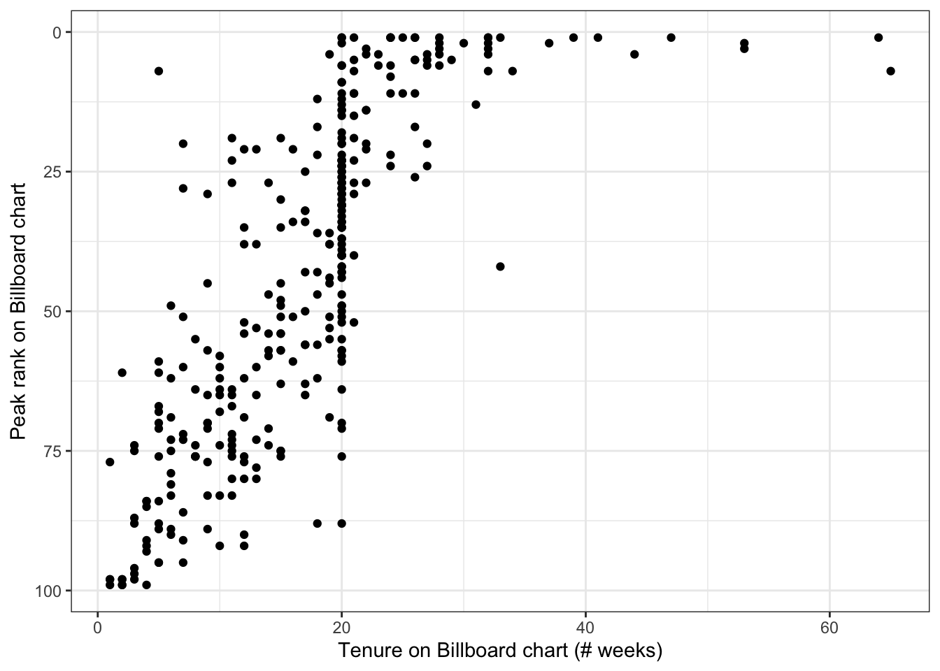
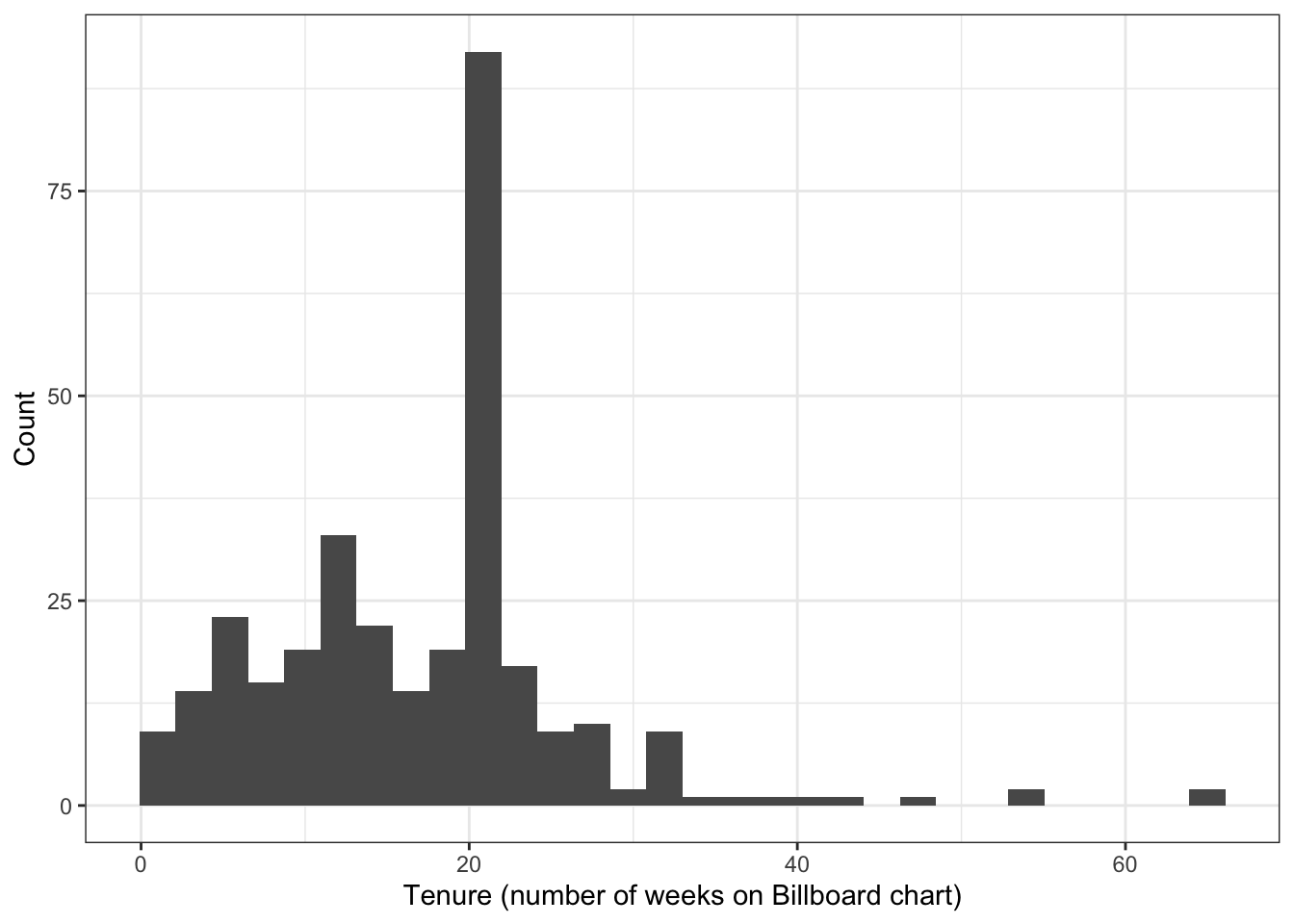
This makes sense: songs with long-tenure on the chart also reach a higher peak rank, on average. But this also reveals something unexpected: we see an over-abundance of songs with a 20-week lifetime on the charts. Let’s take a closer look at some of the examples with a 20-week tenure:
song_summary %>% filter(tenure == 20) %>% print(n = 5)# A tibble: 80 × 4
# Groups: artist [72]
artist track peak_rank tenure
<chr> <chr> <dbl> <dbl>
1 3 Doors Down Loser 55 20
2 98^0 Give Me Just One Nig... 2 20
3 Aaliyah I Don't Wanna 35 20
4 Adams, Yolanda Open My Heart 57 20
5 Alice Deejay Better Off Alone 27 20
# ℹ 75 more rowsdat %>%
filter(artist == 'Aaliyah' & track == "I Don't Wanna") %>%
print(n = Inf)# A tibble: 20 × 8
artist track date.entered week rank year_entered week_num date_rank
<chr> <chr> <date> <chr> <dbl> <dbl> <dbl> <date>
1 Aaliyah I Don't Wa… 2000-01-29 wk1 84 2000 1 2000-01-29
2 Aaliyah I Don't Wa… 2000-01-29 wk2 62 2000 2 2000-02-05
3 Aaliyah I Don't Wa… 2000-01-29 wk3 51 2000 3 2000-02-12
4 Aaliyah I Don't Wa… 2000-01-29 wk4 41 2000 4 2000-02-19
5 Aaliyah I Don't Wa… 2000-01-29 wk5 38 2000 5 2000-02-26
6 Aaliyah I Don't Wa… 2000-01-29 wk6 35 2000 6 2000-03-04
7 Aaliyah I Don't Wa… 2000-01-29 wk7 35 2000 7 2000-03-11
8 Aaliyah I Don't Wa… 2000-01-29 wk8 38 2000 8 2000-03-18
9 Aaliyah I Don't Wa… 2000-01-29 wk9 38 2000 9 2000-03-25
10 Aaliyah I Don't Wa… 2000-01-29 wk10 36 2000 10 2000-04-01
11 Aaliyah I Don't Wa… 2000-01-29 wk11 37 2000 11 2000-04-08
12 Aaliyah I Don't Wa… 2000-01-29 wk12 37 2000 12 2000-04-15
13 Aaliyah I Don't Wa… 2000-01-29 wk13 38 2000 13 2000-04-22
14 Aaliyah I Don't Wa… 2000-01-29 wk14 49 2000 14 2000-04-29
15 Aaliyah I Don't Wa… 2000-01-29 wk15 61 2000 15 2000-05-06
16 Aaliyah I Don't Wa… 2000-01-29 wk16 63 2000 16 2000-05-13
17 Aaliyah I Don't Wa… 2000-01-29 wk17 62 2000 17 2000-05-20
18 Aaliyah I Don't Wa… 2000-01-29 wk18 67 2000 18 2000-05-27
19 Aaliyah I Don't Wa… 2000-01-29 wk19 83 2000 19 2000-06-03
20 Aaliyah I Don't Wa… 2000-01-29 wk20 86 2000 20 2000-06-10# dat %>%
# filter(artist == 'Avant' & track == "Separated") %>%
# print(n = Inf) # removed this, **TO DO clean up laterWe don’t see any obvious signs of error in a couple of examples here. So what’s going on with the cluster of 20-week-olds? Doing some investigations, this site reveals what’s going on:
“See the heavy dropoff on the 20th week starting in 1991? In an attempt to increase diversity and promote newer artists and songs, Billboard changed their methodology, removing tracks that had been on the Hot 100 for twenty consecutive weeks and slipped below the 50th position. These songs, called “recurrents,” were then moved to their own chart in 1991, the Hot 100 Recurrent.”
So tenure was truncated for songs that were > 20 weeks old, and went below rank 50.
Let’s visualize the life and death of some of the longest-running hit songs:
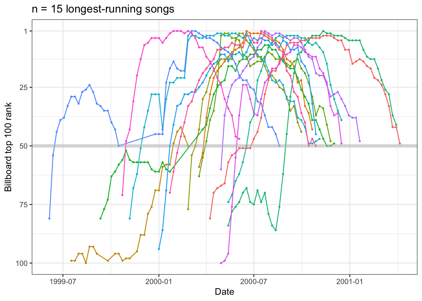
Nearly all of the long-running songs reach #1 on the charts. We see a pretty consistent pattern of rise and fall for these long-running songs.
We can also see that there are a few hits that get a “second life” (they rise and plateau or fall, then rise dramatically again to #1). Why might that be?
We also see the effects of Billboard’s (other) recurrents chart here, because we see how common it is for long-running songs to get killed off with a final rank just around 50. I added grey line to highlight this. We would not expect that to occur by chance! The abundance of death at ~50 is another sign of the recurrent rule, described in the section above.
… in progress / to be continued …