Independent Exploratory Data Analysis - Boat Speed Estimation with Underwater Acoustic Monitoring

Author

Affiliation

Steven Robinson

Department of Geography & Environmental Studies, Carleton University

Published

April 17, 2025

Modified

September 9, 2025

Background

For my M.Sc. Geography thesis, I am studying recreational boat traffic and the impacts of boat wakes in the Rideau Waterway in Eastern Ontario. Wakes – the series of waves produced by a moving vessel – can cause an array of potentially harmful impacts to freshwater environments and biological communities, including shoreline erosion, habitat degradation, wildlife disturbance, and diminished water quality (Gabel et al., 2017). Boating is more popular than ever before, and boat-related recreation is increasingly recognized as a source of disturbance to inland waterways (Schafft et al., 2021).

My research is designed in partnership with Parks Canada, the managing authority of nine navigable waterways in Canada, and stems from the “Freshwater Missions” NSERC Alliance Grant led by Dr. Steven Cooke (Carleton University). Freshwater Missions was a collaborative initiative that brought together Ontario-based universities, conservation authorities, federal agencies, and stewardship organizations to study anthropogenic pressures on freshwater systems and to identify management strategies to reduce these pressures. A specific objective was to develop predictive models of how boat type and speed of navigation influence wake generation.

Unfortunately, obtaining reliable data on navigation speeds of recreational vessel traffic remains a practical challenge (Forlini et al., 2021). Thus, there is need to develop reliable and cost-effective methods for estimating boat speed to better understand the relationship vessel speed and wake generation across different of boat types. Improved speed estimation would also help address waterway management questions, such as:

What speed restrictions would most effectively reduce the amount of wake energy reaching shorelines?
Are boaters adhering to posted speed restrictions?

Common speed detection devices used by enforcement agencies (e.g., radar, laser, and LiDAR instruments) have reduced accuracy when used to track watercraft, especially small pleasurecraft. Further, these approaches are costly and difficult to automate - limiting the scope of a sampling plan. Here, I investigate a novel, cost-effective, and fully autonomous method for estimating boat speed using passive underwater acoustic recordings.

Goal and Research Questions

The goal of this exploratory data analysis (EDA) is to develop and test an automated workflow for boat speed estimation using underwater acoustic recordings. My supervisor (Dr. Jesse Vermaire) is interested in studying the underwater soundscape of the Rideau Waterway and we have experimented with underwater microphones (hydrophones) to record biotic sounds and boat noise. Underwater recorders are conveniently inconspicuous and can deployed for long periods.

The research questions to be addressed in this EDA are:

Can underwater acoustic recordings be used to estimate boat speed?
If yes, can a fully automated workflow be developed in R (R Core Team, 2025)?
If yes, is the method reliable enough to be put into practice for the 2025 sampling season?

Required Packages

library(seewave)
library(tuneR)
library(Metrics)
library(tidyverse)
library(knitr)
library(kableExtra)
library(patchwork)

Experimental Design

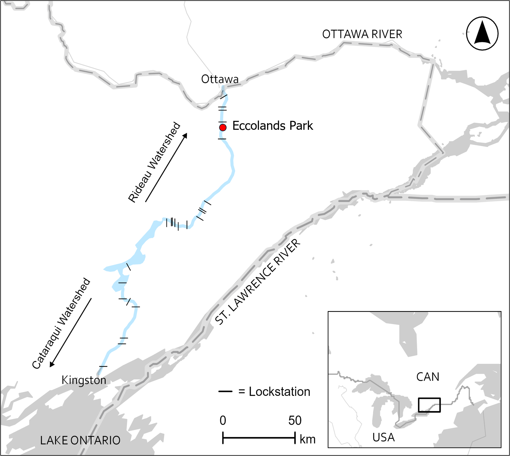
In the fall of 2023 and 2024, we conducted controlled boat trials at Eccolands Park south of Ottawa. The main purpose of these trials was to generate data on wake heights produced by different vessels when operated at variety of speeds and distances from shore, but I also seized the opportunity to experiment with underwater acoustic recorders for boat speed estimation. Figure 1 provides an overview of the Rideau Waterway and experimental design.

Figure 1: Maps of **(A)** the Rideau Waterway and **(B)** experimental setup. Boats were run at a variety of speeds at distances of 30 m, 60 m, and 100 m from the east shore.

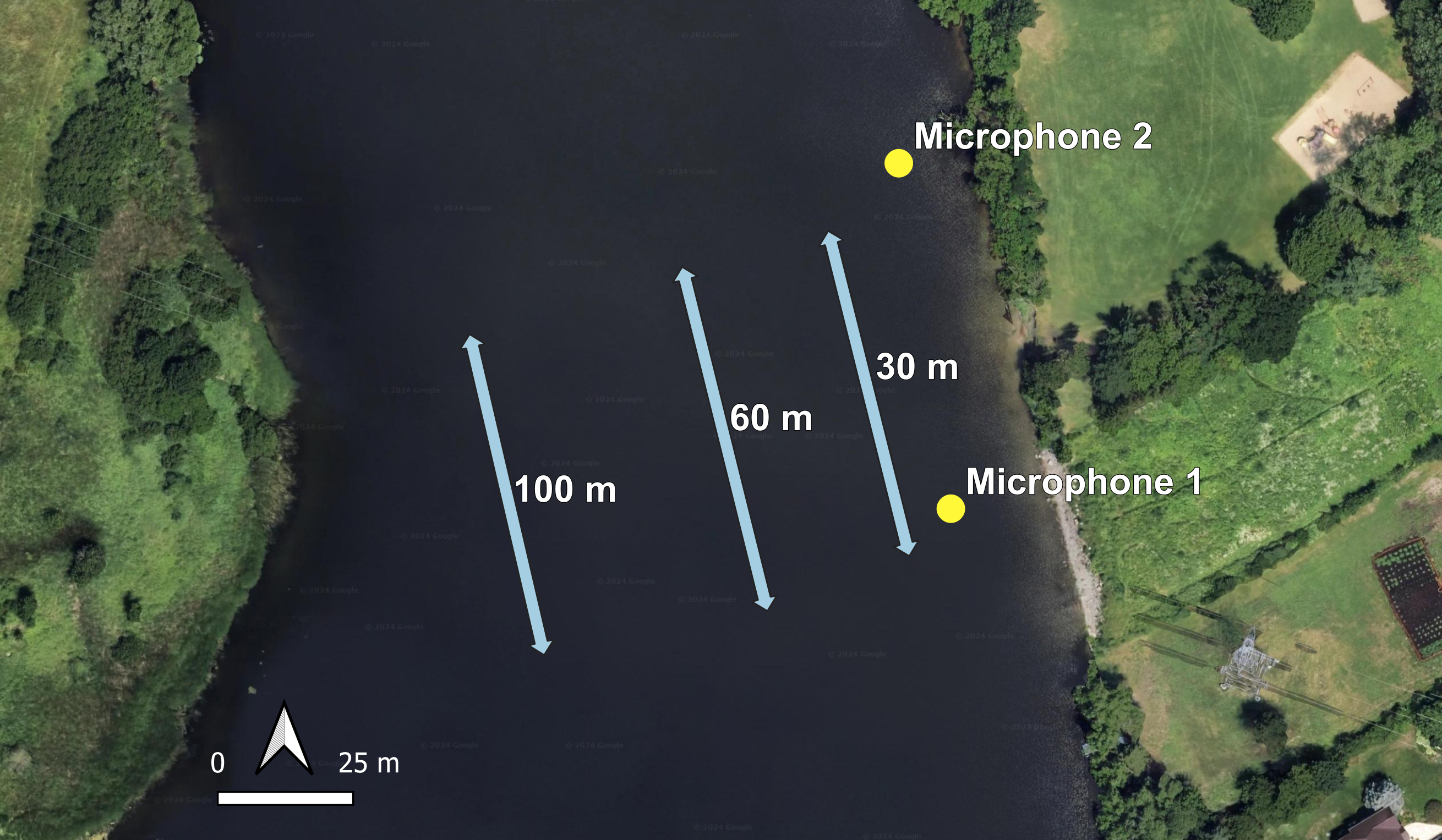
Figure 2 provides a more detailed look at the instrumental setup.

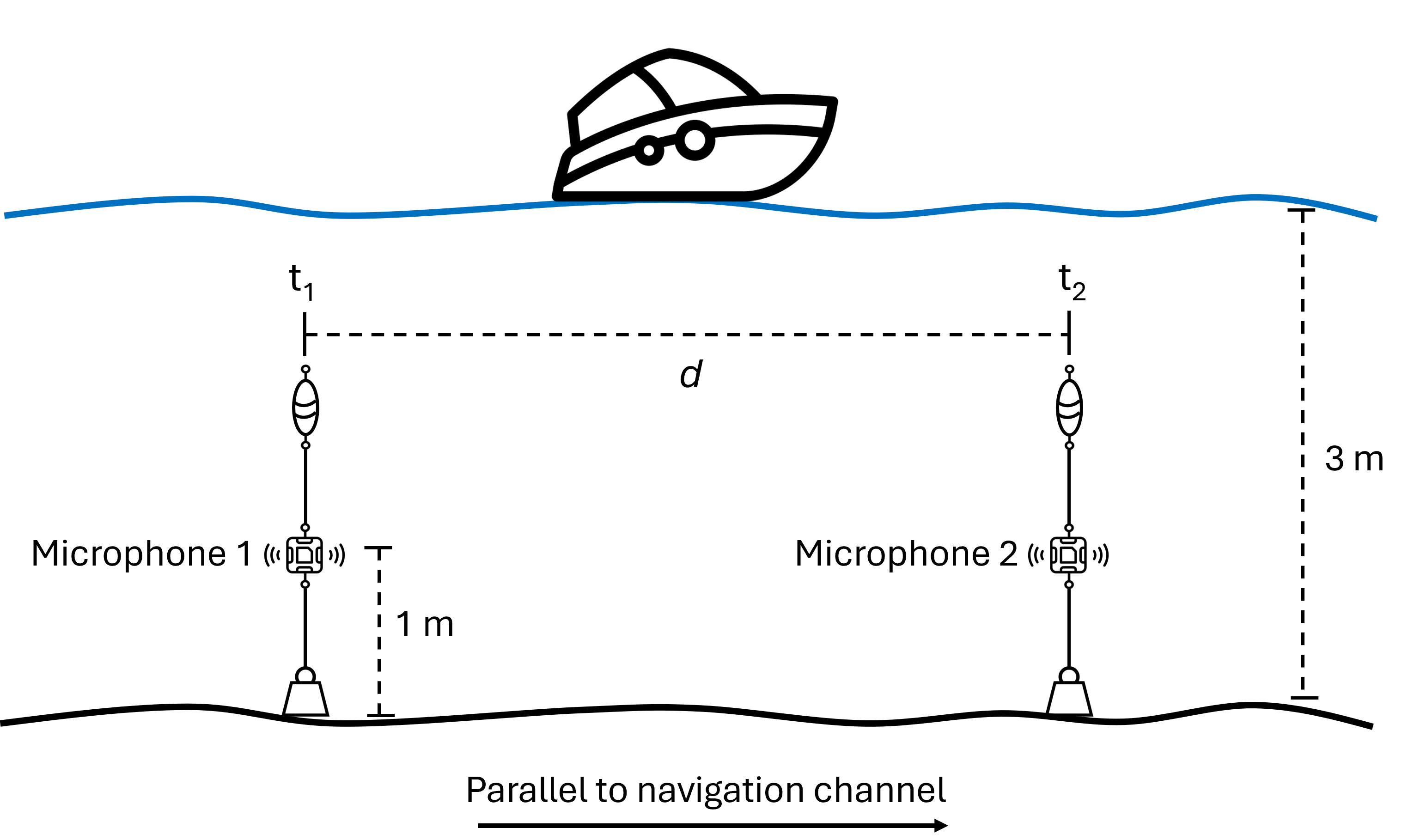
Figure 2: Experimental setup (side view). Acoustic recorders are anchored to the bottom and suspended by subsurface buoys. The time difference between peak sound amplitude at each recorder is used to estimate boat speed.

Two recorders were suspended by underwater buoys in a line parallel to the navigation channel. The distance (d) between the recorders is determined from GPS coordinates. When a boat passes, sound is registered first at one microphone, then the other, and the time interval (𝛥t) between sounds can be used to calculate boat speed with:

\[ v = \frac{d}{\Delta t} \tag{1}\]

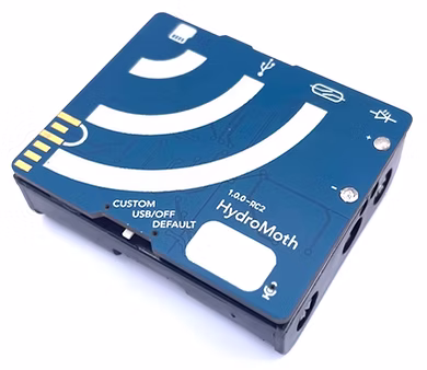
Most commercial underwater acoustic recorders are bloody expensive. Thankfully, an open-source initiative called Open Acoustic Devices recently released a waterproof version of their low-cost AudioMoth device (Hill et al., 2018), which they’ve dubbed HydroMoth (Lamont et al., 2022). My lab picked up a couple HydroMoths (Figure 3) this past summer and they are used for this experiment.

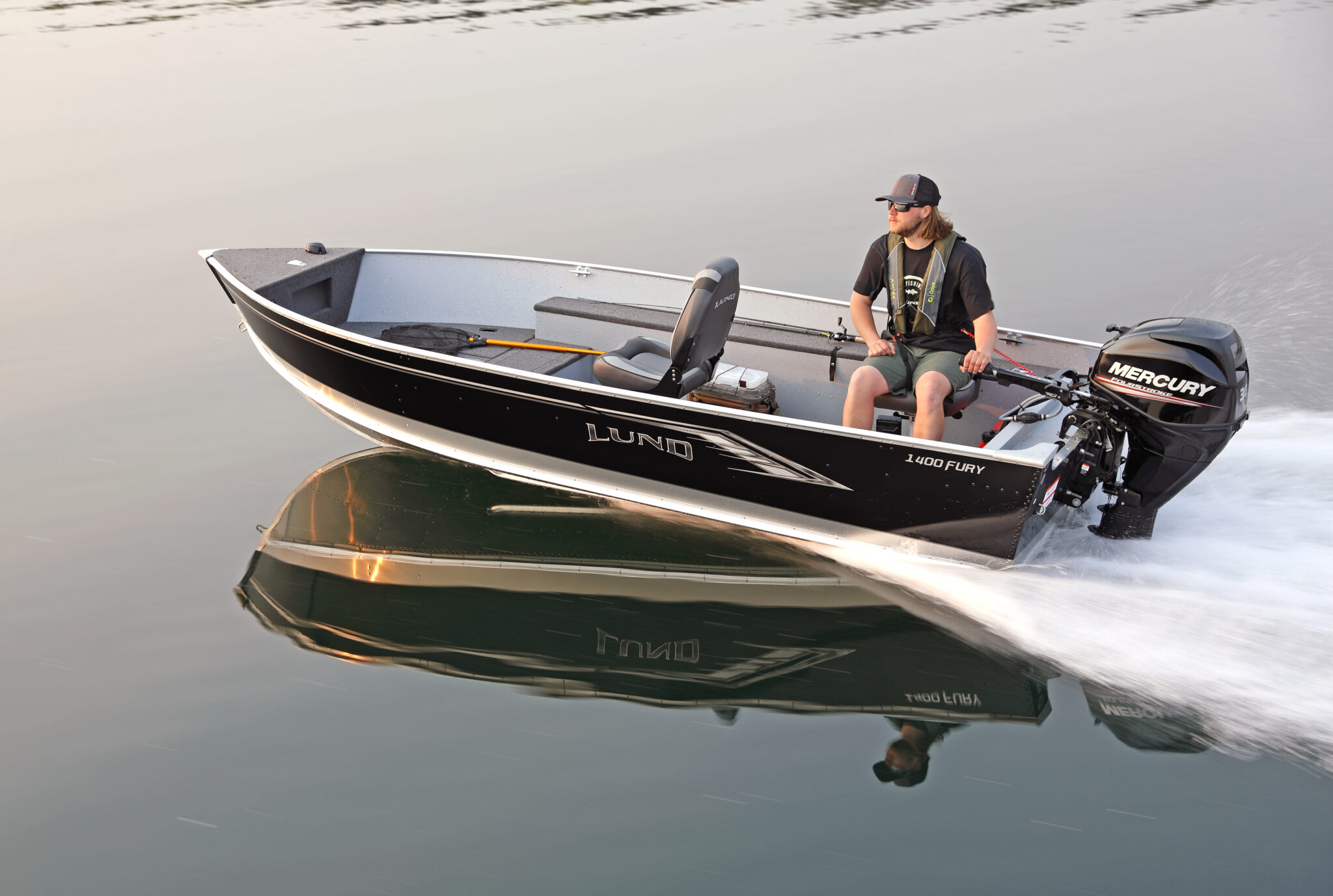
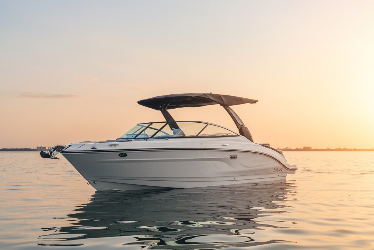
Figure 3: Open Acoustic Devices *HydroMoth* recorder. Don’t forget - you need the waterproof case too.

Three days of trials were selected for method validation (we did a fourth day, but I forgot to press record on one of the mics – whoops!). The boat types used were: 14’ aluminum Lund 1400 Fury; 23’ Ski Nautique Super Air G23 wake surf boat; and 28’ Sea Ray 280 cruiser (Figure 4).

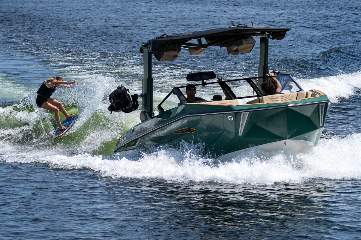
Trials were done late in the season to reduce interference from regular boat traffic. There were 92 controlled boat passes over the three days in this analysis. Passes were performed at 30 meters (m), 60 m and 100 m from shore in upstream and downstream directions, at speeds ranging from 5 km/h up to 70 km/h. Figure 5 shows one of the wake boat passes.

Figure 5: Wake surf boat pass at 18 km/h and 30 m from shore with port-side ballast filled. Sept 25, 2024.

Datasets

Three datasets are used in this analysis:

‘Ground truth’ boat speed observations measured by onboard GPS speedometers and boat pass times recorded by observers onshore. This dataset is transcribed from field notes (Table 1);
Speed estimate results from manual analysis in Excel (Table 2); and
Speed estimate results from automated analysis generated by a for-loop in R (Table 3).

The focus of this EDA is on the automated analysis, though the manual results will be included here and there, especially for error analysis towards the end.

# Boat speed observations 
obs <- read_csv("2024_experimental_obs.csv")

obs |> 
  mutate(across(where(is.numeric), ~ round(.x, 1))) |> 
  kable() |> 
  kable_styling(full_width = FALSE) |> 
  scroll_box(height = "400px")

Table 1: Ground truth boat pass observations used for validation.

date	event	time_NDA	time_SR	boat_dist_m	speed_kmh	dir	boat_type	shaper	mic_dist_m	notes
20240920	1	14:09:00	NA	100	10	up	alum	NA	62.1	NA
20240920	2	14:24:31	NA	100	10	down	alum	NA	62.1	NA
20240920	3	14:34:12	NA	100	10	up	alum	NA	62.1	NA
20240920	4	14:42:20	NA	100	10	down	alum	NA	62.1	NA
20240920	5	14:49:55	NA	100	20	up	alum	NA	62.1	NA
20240920	6	14:59:35	NA	100	20	down	alum	NA	62.1	NA
20240920	7	15:11:35	NA	100	17	up	alum	NA	62.1	NA
20240920	8	15:14:00	NA	NA	NA	NA	NA	NA	62.1	not our boat
20240920	9	15:20:44	NA	100	21	down	alum	NA	62.1	NA
20240920	10	15:26:55	NA	100	30	up	alum	NA	62.1	NA
20240920	11	15:41:50	NA	100	27	down	alum	NA	62.1	NA
20240920	12	15:48:48	NA	100	28	up	alum	NA	62.1	NA
20240920	13	15:50:34	NA	NA	NA	NA	NA	NA	62.1	not our boat
20240920	14	15:58:15	NA	60	10	down	alum	NA	62.1	NA
20240920	15	16:06:08	NA	60	10	up	alum	NA	62.1	NA
20240920	16	16:09:55	NA	NA	NA	NA	NA	NA	62.1	not our boat
20240925	1	12:48:39	12:49:00	100	6	up	wake	off	68.7	no wake
20240925	2	12:53:22	12:53:20	100	6	down	wake	off	68.7	no wake
20240925	3	12:56:30	12:56:50	60	5.5	up	wake	off	68.7	NA
20240925	4	12:59:00	12:59:10	60	6	down	wake	off	68.7	NA
20240925	5	13:02:44	13:02:45	30	6	up	wake	off	68.7	NA
20240925	6	13:05:08	13:05:20	30	6	down	wake	off	68.7	NA
20240925	7	13:08:48	13:08:50	100	27	up	wake	off	68.7	NA
20240925	8	13:15:07	13:14:55	100	27	down	wake	off	68.7	NA
20240925	9	13:18:23	13:18:10	NA	S	down	cruiser	NA	68.7	not our boat
20240925	10	13:23:40	13:23:50	100	18	up	wake	on	68.7	NA
20240925	11	13:30:12	13:30:12	100	18	down	wake	on	68.7	NA
20240925	12	13:36:59	13:36:59	60	18	up	wake	on	68.7	NA
20240925	13	13:43:45	13:43:45	60	18	down	wake	on	68.7	NA
20240925	14	13:51:34	13:51:34	30	18	up	wake	on	68.7	NA
20240925	15	13:58:07	13:57:07	30	18	down	wake	on	68.7	NA
20240925	16	14:04:26	14:04:20	30	27	up	wake	on	68.7	NA
20240925	17	14:12:02	14:12:02	30	27	down	wake	on	68.7	NA
20240925	18	14:19:12	14:19:12	60	27	up	wake	on	68.7	NA
20240925	19	14:24:59	14:24:59	60	27	down	wake	on	68.7	NA
20240925	20	14:29:45	14:29:45	60	27	up	wake	on	68.7	NA
20240925	21	14:33:39	14:33:39	60	27	down	wake	on	68.7	NA
20240925	22	14:41:56	14:42:00	100	10	up	wake	on	68.7	NA
20240925	23	14:48:40	14:48:45	100	10	down	wake	on	68.7	NA
20240925	24	14:52:55	14:52:55	100	27	up	wake	on	68.7	NA
20240925	25	14:59:24	14:59:28	100	27	down	wake	on	68.7	NA
20240925	26	15:07:05	15:07:05	60	10	up	wake	on	68.7	NA
20240925	27	15:12:34	15:12:34	60	10	down	wake	on	68.7	NA
20240925	28	15:18:52	15:18:57	30	10	up	wake	on	68.7	NA
20240925	29	15:24:32	15:24:40	30	10	down	wake	on	68.7	NA
20240925	30	15:33:21	15:33:21	100	18	up	wake	off	68.7	NA
20240925	31	15:40:09	15:40:09	100	18	down	wake	off	68.7	NA
20240925	32	15:47:43	15:47:43	60	18	up	wake	off	68.7	NA
20240925	33	15:55:21	15:55:21	60	18	down	wake	off	68.7	NA
20240925	34	16:02:25	16:02:25	30	18	up	wake	off	68.7	NA
20240925	35	16:08:53	16:08:10	30	18	down	wake	off	68.7	RBR tipped
20240925	36	16:15:35	16:15:35	60	27	up	wake	off	68.7	NA
20240925	37	16:22:03	16:22:03	60	27	down	wake	off	68.7	NA
20240925	38	16:28:28	16:28:28	30	27	up	wake	off	68.7	NA
20240925	39	16:34:51	16:34:51	30	27	down	wake	off	68.7	NA
20240925	40	16:37:17	16:37:17	65	55	up	wake	off	68.7	NA
20240925	41	16:43:00	16:43:20	30	57	down	wake	off	68.7	NA
20241004	1	NA	11:58:30	65	S	up	cruiser	NA	64.3	not our boat
20241004	2	NA	12:08:40	100	9.7	up	cruiser	NA	64.3	NA
20241004	3	NA	12:11:15	65	S	down	cruiser	NA	64.3	not our boat
20241004	4	NA	12:20:30	100	9.9	down	cruiser	NA	64.3	NA
20241004	5	NA	12:33:20	60	9.7	up	cruiser	NA	64.3	NA
20241004	6	NA	12:40:27	60	9.7	down	cruiser	NA	64.3	NA
20241004	7	NA	12:44:55	50	M	up	runabout	NA	64.3	not our boat
20241004	8	NA	12:46:25	80	M	up	pontoon	NA	64.3	not our boat
20241004	9	NA	12:50:40	30	9.5	up	cruiser	NA	64.3	NA
20241004	10	NA	12:56:15	40	S	down	runabout	NA	64.3	not our boat
20241004	11	NA	12:58:51	95	F	up	ski	NA	64.3	not our boat
20241004	12	NA	13:03:16	30	9.3	down	cruiser	NA	64.3	NA
20241004	13	NA	13:09:48	30	21.7	up	cruiser	NA	64.3	Big!
20241004	14	NA	13:15:29	30	20.1	down	cruiser	NA	64.3	Big!
20241004	15	NA	13:23:24	30	32.1	up	cruiser	NA	64.3	NA
20241004	16	NA	13:30:26	30	30.9	down	cruiser	NA	64.3	NA
20241004	17	NA	13:40:35	30	48.2	up	cruiser	NA	64.3	NA
20241004	18	NA	13:53:23	30	50.7	down	cruiser	NA	64.3	NA
20241004	19	NA	13:55:10	85	M	up	alum	NA	64.3	not our boat
20241004	20	NA	14:00:57	60	27.8	up	cruiser	NA	64.3	NA
20241004	21	NA	14:06:00	60	21.5	down	cruiser	NA	64.3	NA
20241004	22	NA	14:13:10	60	21.6	up	cruiser	NA	64.3	NA
20241004	23	NA	14:19:28	60	60	down	cruiser	NA	64.3	NA
20241004	24	NA	14:24:51	60	59.5	up	cruiser	NA	64.3	NA
20241004	25	NA	14:32:15	100	19.7	down	cruiser	NA	64.3	NA
20241004	26	NA	14:38:06	100	19.9	up	cruiser	NA	64.3	NA
20241004	27	NA	14:43:46	100	59.5	down	cruiser	NA	64.3	NA
20241004	28	NA	14:46:24	65	NA	down	alum	NA	64.3	not our boat
20241004	29	NA	14:52:18	100	62.1	up	cruiser	NA	64.3	NA
20241004	30	NA	14:56:50	60	61.7	down	cruiser	NA	64.3	NA
20241004	31	NA	15:03:03	30	61.1	up	cruiser	NA	64.3	NA
20241004	32	NA	15:11:12	60	NA	down	ski	NA	64.3	not our boat
20241004	33	NA	15:14:38	30	67.8	down	cruiser	NA	64.3	NA
20241004	34	NA	15:29:05	50	S	up	runabout	NA	64.3	not our boat
20241004	35	NA	15:33:00	30	11.2	up	cruiser	NA	64.3	NA
20241004	36	NA	15:37:21	30	11.5	down	cruiser	NA	64.3	NA
20241004	37	NA	15:43:00	30	18.6	up	cruiser	NA	64.3	NA
20241004	38	NA	15:48:43	30	23.1	down	cruiser	NA	64.3	NA
20241004	39	NA	15:55:13	60	11.6	up	cruiser	NA	64.3	NA
20241004	40	NA	16:01:35	60	11.6	down	cruiser	NA	64.3	NA
20241004	41	NA	16:05:37	60	22	up	cruiser	NA	64.3	NA
20241004	42	NA	16:10:24	100	64.1	down	cruiser	NA	64.3	NA
20241004	43	NA	16:15:10	100	67.1	up	cruiser	NA	64.3	NA
20241004	44	NA	16:20:50	100	22	down	cruiser	NA	64.3	NA
20241004	45	NA	16:24:48	35	S	down	runabout	NA	64.3	not our boat
20241004	46	NA	16:30:05	100	20.9	up	cruiser	NA	64.3	NA
20241004	47	NA	16:36:31	100	10.5	down	cruiser	NA	64.3	NA
20241004	48	NA	16:44:21	100	10.7	up	cruiser	NA	64.3	NA
20241004	49	NA	16:50:10	60	23.9	down	runabout	NA	64.3	NA
20241004	50	NA	16:53:22	60	F	down	cruiser	NA	64.3	knee boarder
20241004	51	NA	16:56:36	60	59.9	up	cruiser	NA	64.3	NA
20241004	52	NA	16:58:25	60	F	up	runabout	NA	64.3	not our boat
20241009	1	NA	11:45:09	100	9.5	up	bass	NA	33.8	NA
20241009	2	NA	11:49:20	100	9.8	down	bass	NA	33.8	NA
20241009	3	NA	11:54:15	100	19	up	bass	NA	33.8	NA
20241009	4	NA	11:59:22	100	17.3	down	bass	NA	33.8	NA
20241009	5	NA	12:03:50	100	32	up	bass	NA	33.8	NA
20241009	6	NA	12:08:17	100	32	down	bass	NA	33.8	NA
20241009	7	NA	12:13:00	100	60.1	up	bass	NA	33.8	NA
20241009	8	NA	12:17:30	100	60.5	down	bass	NA	33.8	NA
20241009	9	NA	12:21:57	60	9	up	bass	NA	33.8	NA
20241009	10	NA	12:25:40	60	9.3	down	bass	NA	33.8	NA
20241009	11	NA	12:29:30	60	20	up	bass	NA	33.8	NA
20241009	12	NA	12:34:09	60	18	down	bass	NA	33.8	NA
20241009	13	NA	12:39:28	60	17.5	up	bass	NA	33.8	NA
20241009	14	NA	12:44:22	60	17.5	down	bass	NA	33.8	NA
20241009	15	NA	12:48:20	60	30	up	bass	NA	33.8	NA
20241009	16	NA	12:52:20	60	31	down	bass	NA	33.8	NA
20241009	17	NA	12:57:42	60	58	up	bass	NA	33.8	NA
20241009	18	NA	13:02:25	60	60	down	bass	NA	33.8	NA
20241009	19	NA	13:06:50	30	9.6	up	bass	NA	33.8	NA
20241009	20	NA	13:09:09	30	9.6	down	bass	NA	33.8	NA
20241009	21	NA	13:12:01	30	17.4	up	bass	NA	33.8	NA
20241009	22	NA	13:17:50	30	18	down	bass	NA	33.8	NA
20241009	23	NA	13:21:47	30	35	up	bass	NA	33.8	NA
20241009	24	NA	13:25:59	30	29	down	bass	NA	33.8	NA
20241009	25	NA	13:29:45	30	60	up	bass	NA	33.8	NA
20241009	26	NA	13:33:19	30	58	down	bass	NA	33.8	NA
20241009	27	NA	13:37:55	100	9.3	up	bass	NA	33.8	NA
20241009	28	NA	13:41:25	100	9.8	down	bass	NA	33.8	NA
20241009	29	NA	13:46:30	100	17.5	up	bass	NA	33.8	NA
20241009	30	NA	13:50:45	100	18	down	bass	NA	33.8	NA
20241009	31	NA	13:54:15	100	31	up	bass	NA	33.8	NA
20241009	32	NA	13:57:50	100	30	down	bass	NA	33.8	NA
20241009	33	NA	14:01:30	100	60	up	bass	NA	33.8	NA
20241009	34	NA	14:05:15	100	60	down	bass	NA	33.8	NA
20241009	35	NA	14:09:30	60	9.5	up	bass	NA	33.8	NA
20241009	36	NA	14:12:49	60	9.5	down	bass	NA	33.8	NA
20241009	37	NA	14:16:15	60	33	up	bass	NA	33.8	NA
20241009	38	NA	14:20:08	60	30	up	bass	NA	33.8	NA
20241009	39	NA	14:23:52	60	58	down	bass	NA	33.8	NA
20241009	40	NA	14:26:49	60	60	up	bass	NA	33.8	NA
20241009	41	NA	14:29:52	NA	S	up	yacht	NA	33.8	Le Boat
20241009	42	NA	14:32:47	30	9.6	up	bass	NA	33.8	NA
20241009	43	NA	14:36:35	30	9.5	down	bass	NA	33.8	NA
20241009	44	NA	14:39:08	30	16.5	up	bass	NA	33.8	NA
20241009	45	NA	14:42:58	30	18	down	bass	NA	33.8	NA
20241009	46	NA	14:46:26	30	30	up	bass	NA	33.8	NA
20241009	47	NA	14:50:33	30	31	down	bass	NA	33.8	NA
20241009	48	NA	14:53:55	30	57	up	bass	NA	33.8	NA
20241009	49	NA	14:57:50	30	59.5	down	bass	NA	33.8	NA

# Manual boat speed estimates
man <- read_csv("man_est.csv")

man |> 
  mutate(across(where(is.numeric), ~ round(.x, 1))) |>
  kable() |> 
  kable_styling(full_width = FALSE) |> 
  scroll_box(height = "400px")

Table 2: Boat speed estimates from manual analysis.

date	time	dist_m	pred_kmh	obs_kmh	type	notes
9/20/2024	14:10:30	100	5.3	10	alum	not our boat?
9/20/2024	14:25:09	100	6.6	10	alum	NA
9/20/2024	14:34:22	100	5.4	10	alum	not our boat
9/20/2024	14:42:22	100	6.6	10	alum	not out boat
9/20/2024	14:49:58	100	13.5	20	alum	NA
9/20/2024	14:59:40	100	10.9	20	alum	not our boat
9/20/2024	15:11:34	100	16.3	17	alum	not our boat
9/20/2024	15:14:18	#N/A	9.0	#N/A	alum	NA
9/20/2024	15:20:42	100	15.0	21	alum	NA
9/20/2024	15:26:58	100	13.7	30	alum	NA
9/20/2024	15:41:50	100	18.5	27	alum	NA
9/20/2024	15:48:50	100	21.3	28	alum	NA
9/20/2024	15:50:22	#N/A	35.5	#N/A	alum	not our boat?
9/20/2024	15:58:18	60	8.8	10	alum	NA
9/20/2024	16:06:16	60	9.6	10	alum	?
9/20/2024	16:09:54	#N/A	26.3	#N/A	alum	NA
9/20/2024	16:12:59	#N/A	26.9	#N/A	alum	not our boat
9/20/2024	16:17:50	#N/A	23.8	#N/A	alum	NA
9/20/2024	16:18:36	#N/A	21.9	#N/A	alum	NA
9/25/2024	12:48:58	100	4.6	6	wake	NA
9/25/2024	12:53:37	100	5.2	6	wake	NA
9/25/2024	12:56:55	60	5.9	5.5	wake	NA
9/25/2024	12:59:14	60	5.6	6	wake	NA
9/25/2024	13:02:52	30	6.7	6	wake	NA
9/25/2024	13:05:27	30	6.2	6	wake	NA
9/25/2024	13:08:51	100	35.3	27	wake	Not our boat
9/25/2024	13:14:54	100	27.5	27	wake	NA
9/25/2024	13:17:57	#N/A	7.5	#N/A	wake	NA
9/25/2024	13:23:52	100	18.2	18	wake	NA
9/25/2024	13:30:01	100	21.5	18	wake	not out boat
9/25/2024	13:37:08	60	16.6	18	wake	NA
9/25/2024	13:43:56	60	19.5	18	wake	not out boat
9/25/2024	13:51:41	30	17.8	18	wake	NA
9/25/2024	13:58:14	30	19.5	18	wake	NA
9/25/2024	14:04:27	30	27.5	27	wake	NA
9/25/2024	14:12:06	30	25.8	27	wake	NA
9/25/2024	14:19:12	60	22.1	27	wake	NA
9/25/2024	14:25:06	60	38.0	27	wake	NA
9/25/2024	14:29:57	60	17.9	27	wake	NA
9/25/2024	14:33:44	60	25.8	27	wake	NA
9/25/2024	14:41:58	100	11.3	10	wake	NA
9/25/2024	14:48:49	100	10.7	10	wake	NA
9/25/2024	14:52:59	100	19.5	27	wake	Not our boat
9/25/2024	14:59:30	100	28.1	27	wake	NA
9/25/2024	15:07:09	60	8.2	10	wake	NA
9/25/2024	15:12:42	60	10.3	10	wake	NA
9/25/2024	15:18:58	30	10.3	10	wake	NA
9/25/2024	15:24:40	30	10.8	10	wake	Not out boat
9/25/2024	15:33:30	100	22.7	18	wake	NA
9/25/2024	15:40:12	100	15.1	18	wake	NA
9/25/2024	15:47:48	60	17.7	18	wake	Not our boat
9/25/2024	15:55:26	60	17.7	18	wake	NA
9/25/2024	16:02:30	30	16.5	18	wake	NA
9/25/2024	16:08:57	30	19.0	18	wake	NA
9/25/2024	16:15:39	60	20.6	27	wake	NA
9/25/2024	16:22:08	60	24.7	27	wake	NA
9/25/2024	16:28:30	30	30.9	27	wake	NA
9/25/2024	16:34:54	30	27.5	27	wake	NA
9/25/2024	16:37:40	65	46.7	55	wake	NA
9/25/2024	16:43:11	30	49.5	57	wake	NA
9/25/2024	16:59:30	#N/A	30.9	#N/A	wake	NA
10/4/2024	12:00:42	#N/A	0.8	#N/A	cruiser	NA
10/4/2024	12:08:10	100	4.5	9.7	cruiser	NA
10/4/2024	12:11:15	#N/A	9.9	#N/A	cruiser	NA
10/4/2024	12:20:36	100	12.7	9.9	cruiser	NA
10/4/2024	12:33:22	60	11.5	9.7	cruiser	NA
10/4/2024	12:39:34	#N/A	61.3	#N/A	cruiser	NA
10/4/2024	12:40:29	60	10.7	9.7	cruiser	NA
10/4/2024	12:44:51	#N/A	15.8	#N/A	cruiser	NA
10/4/2024	12:46:21	#N/A	15.7	#N/A	cruiser	NA
10/4/2024	12:50:35	30	10.4	9.5	cruiser	NA
10/4/2024	12:56:16	#N/A	8.9	#N/A	cruiser	NA
10/4/2024	12:58:49	#N/A	24.9	#N/A	cruiser	NA
10/4/2024	13:03:26	30	11.3	9.3	cruiser	NA
10/4/2024	13:09:42	30	21.1	21.7	cruiser	NA
10/4/2024	13:15:32	30	23.5	20.1	cruiser	NA
10/4/2024	13:23:28	30	30.2	32.1	cruiser	NA
10/4/2024	13:30:28	30	45.9	30.9	cruiser	NA
10/4/2024	13:33:48	#N/A	576.7	#N/A	cruiser	NA
10/4/2024	13:40:26	30	64.9	48.2	cruiser	NA
10/4/2024	13:50:27	#N/A	147.8	#N/A	cruiser	NA
10/4/2024	13:53:24	30	63.7	50.7	cruiser	NA
10/4/2024	13:55:11	#N/A	16.6	#N/A	cruiser	NA
10/4/2024	14:00:56	60	16.5	27.8	cruiser	NA
10/4/2024	14:06:02	60	28.7	21.5	cruiser	NA
10/4/2024	14:13:16	60	25.7	21.6	cruiser	NA
10/4/2024	14:19:27	60	73.8	60	cruiser	NA
10/4/2024	14:24:55	60	78.2	59.5	cruiser	NA
10/4/2024	14:32:17	100	38.2	19.7	cruiser	NA
10/4/2024	14:38:00	100	20.9	19.9	cruiser	NA
10/4/2024	14:43:49	100	46.0	59.5	cruiser	NA
10/4/2024	14:46:24	#N/A	29.4	#N/A	cruiser	NA
10/4/2024	14:52:07	100	42.3	62.1	cruiser	NA
10/4/2024	14:56:51	60	76.1	61.7	cruiser	NA
10/4/2024	15:03:04	30	91.0	61.1	cruiser	NA
10/4/2024	15:11:32	#N/A	582.6	#N/A	cruiser	NA
10/4/2024	15:14:38	30	88.3	67.8	cruiser	NA
10/4/2024	15:29:02	#N/A	14.0	#N/A	cruiser	NA
10/4/2024	15:33:04	30	18.1	11.2	cruiser	NA
10/4/2024	15:37:25	30	19.0	11.5	cruiser	NA
10/4/2024	15:43:00	30	33.7	18.6	cruiser	NA
10/4/2024	15:48:40	30	32.8	23.1	cruiser	NA
10/4/2024	15:55:09	60	14.5	11.6	cruiser	NA
10/4/2024	16:01:34	60	26.8	11.6	cruiser	NA
10/4/2024	16:05:37	60	22.3	22	cruiser	NA
10/4/2024	16:10:23	100	120.5	64.1	cruiser	NA
10/4/2024	16:15:09	100	51.9	67.1	cruiser	NA
10/4/2024	16:20:48	100	35.4	22	cruiser	NA
10/4/2024	16:24:52	#N/A	15.5	#N/A	cruiser	NA
10/4/2024	16:30:03	100	15.9	20.9	cruiser	NA
10/4/2024	16:36:21	100	19.6	10.5	cruiser	NA
10/4/2024	16:44:32	100	11.3	10.7	cruiser	NA
10/4/2024	16:50:10	60	43.7	23.9	cruiser	NA
10/4/2024	16:53:18	#N/A	56.8	#N/A	cruiser	NA
10/4/2024	16:56:37	60	126.7	59.9	cruiser	NA
10/4/2024	16:58:25	#N/A	69.1	#N/A	cruiser	NA
10/4/2024	16:49:57	#N/A	0.4	#N/A	cruiser	NA

# Automatic boat speed estimates
auto <- read_csv("auto_est.csv")

auto |>
  mutate(across(where(is.numeric), ~ round(.x, 1))) |> 
  kable() |> 
  kable_styling(full_width = FALSE) |> 
  scroll_box(height = "400px")

Table 3: Boat speed estimates from automated analysis.

event	group_id	group_event	event_time	event_datetime	mic_dist_m	mic_1	mic_2	peak_avg	delta_t_s	speed_ms	speed_kmh	file	file_time
1	1	1	14:08:28	2024-09-20 14:08:28	62.1	651.1	366.6	508.9	284.5	0.2	0.8	20240920_140000.WAV	2024-09-20 14:00:00
2	1	2	14:10:09	2024-09-20 14:10:09	62.1	NA	609.0	NA	NA	NA	NA	20240920_140000.WAV	2024-09-20 14:00:00
3	2	1	14:25:12	2024-09-20 14:25:12	62.1	292.5	332.6	312.5	40.1	1.5	5.6	20240920_142000.WAV	2024-09-20 14:20:00
4	2	2	14:34:25	2024-09-20 14:34:25	62.1	883.5	847.4	865.4	36.1	1.7	6.2	20240920_142000.WAV	2024-09-20 14:20:00
5	3	1	14:42:22	2024-09-20 14:42:22	62.1	122.2	163.3	142.7	41.1	1.5	5.4	20240920_144000.WAV	2024-09-20 14:40:00
6	3	2	14:49:58	2024-09-20 14:49:58	62.1	607.0	590.0	598.5	17.0	3.6	13.1	20240920_144000.WAV	2024-09-20 14:40:00
7	3	3	14:59:41	2024-09-20 14:59:41	62.1	1170.0	1193.0	1181.5	23.0	2.7	9.7	20240920_144000.WAV	2024-09-20 14:40:00
8	4	1	15:05:25	2024-09-20 15:05:25	62.1	559.9	91.2	325.5	468.8	0.1	0.5	20240920_150000.WAV	2024-09-20 15:00:00
9	4	2	15:10:35	2024-09-20 15:10:35	62.1	711.2	558.9	635.1	152.3	0.4	1.5	20240920_150000.WAV	2024-09-20 15:00:00
10	4	3	15:12:47	2024-09-20 15:12:47	62.1	845.4	690.2	767.8	155.3	0.4	1.4	20240920_150000.WAV	2024-09-20 15:00:00
11	4	4	15:14:34	2024-09-20 15:14:34	62.1	NA	874.5	NA	NA	NA	NA	20240920_150000.WAV	2024-09-20 15:00:00
12	5	1	15:20:47	2024-09-20 15:20:47	62.1	35.1	60.1	47.6	25.0	2.5	8.9	20240920_152000.WAV	2024-09-20 15:20:00
13	5	2	15:26:32	2024-09-20 15:26:32	62.1	427.7	357.6	392.7	70.1	0.9	3.2	20240920_152000.WAV	2024-09-20 15:20:00
14	5	3	15:26:51	2024-09-20 15:26:51	62.1	NA	411.7	NA	NA	NA	NA	20240920_152000.WAV	2024-09-20 15:20:00
15	6	1	15:41:51	2024-09-20 15:41:51	62.1	104.2	119.2	111.7	15.0	4.1	14.9	20240920_154000.WAV	2024-09-20 15:40:00
16	6	2	15:48:53	2024-09-20 15:48:53	62.1	540.9	525.9	533.4	15.0	4.1	14.9	20240920_154000.WAV	2024-09-20 15:40:00
17	6	3	15:50:15	2024-09-20 15:50:15	62.1	625.0	605.0	615.0	20.0	3.1	11.2	20240920_154000.WAV	2024-09-20 15:40:00
18	6	4	15:58:20	2024-09-20 15:58:20	62.1	1086.8	1114.9	1100.8	28.0	2.2	8.0	20240920_154000.WAV	2024-09-20 15:40:00
19	7	1	16:03:29	2024-09-20 16:03:29	62.1	389.7	29.0	209.3	360.6	0.2	0.6	20240920_160000.WAV	2024-09-20 16:00:00
20	7	2	16:07:58	2024-09-20 16:07:58	62.1	590.0	367.6	478.8	222.4	0.3	1.0	20240920_160000.WAV	2024-09-20 16:00:00
21	7	3	16:11:33	2024-09-20 16:11:33	62.1	786.3	601.0	693.7	185.3	0.3	1.2	20240920_160000.WAV	2024-09-20 16:00:00
22	7	4	16:15:21	2024-09-20 16:15:21	62.1	1066.8	775.3	921.0	291.5	0.2	0.8	20240920_160000.WAV	2024-09-20 16:00:00
23	7	5	16:18:19	2024-09-20 16:18:19	62.1	1122.9	1075.8	1099.3	47.1	1.3	4.7	20240920_160000.WAV	2024-09-20 16:00:00
24	7	6	16:18:32	2024-09-20 16:18:32	62.1	NA	1112.9	NA	NA	NA	NA	20240920_160000.WAV	2024-09-20 16:00:00
25	8	1	16:21:27	2024-09-20 16:21:27	62.1	85.1	90.2	87.6	5.0	12.4	44.6	20240920_162000.WAV	2024-09-20 16:20:00
26	8	2	16:22:15	2024-09-20 16:22:15	62.1	140.2	130.2	135.2	10.0	6.2	22.3	20240920_162000.WAV	2024-09-20 16:20:00
27	8	3	16:24:33	2024-09-20 16:24:33	62.1	295.5	251.4	273.5	44.1	1.4	5.1	20240920_162000.WAV	2024-09-20 16:20:00
28	8	4	16:25:27	2024-09-20 16:25:27	62.1	348.6	305.5	327.0	43.1	1.4	5.2	20240920_162000.WAV	2024-09-20 16:20:00
29	8	5	16:26:22	2024-09-20 16:26:22	62.1	425.7	339.6	382.6	86.1	0.7	2.6	20240920_162000.WAV	2024-09-20 16:20:00
30	8	6	16:31:37	2024-09-20 16:31:37	62.1	960.6	434.7	697.7	525.9	0.1	0.4	20240920_162000.WAV	2024-09-20 16:20:00
31	8	7	16:32:01	2024-09-20 16:32:01	62.1	NA	721.2	NA	NA	NA	NA	20240920_162000.WAV	2024-09-20 16:20:00
32	8	8	16:35:53	2024-09-20 16:35:53	62.1	NA	953.6	NA	NA	NA	NA	20240920_162000.WAV	2024-09-20 16:20:00
NA	9	NA	NA	NA	NA	NA	NA	NA	NA	NA	NA	20240920_164000.WAV	2024-09-20 16:40:00
33	10	1	17:12:31	2024-09-20 17:12:31	62.1	741.2	762.3	751.8	21.0	3.0	10.6	20240920_170000.WAV	2024-09-20 17:00:00
34	10	2	17:17:57	2024-09-20 17:17:57	62.1	1079.8	1075.8	1077.8	4.0	15.5	55.8	20240920_170000.WAV	2024-09-20 17:00:00
35	11	1	17:29:00	2024-09-20 17:29:00	62.1	550.9	530.0	540.4	20.9	3.0	10.7	20240920_172000.WAV	2024-09-20 17:20:00
36	11	2	17:31:01	2024-09-20 17:31:01	62.1	662.0	660.2	661.1	1.8	34.4	123.9	20240920_172000.WAV	2024-09-20 17:20:00
37	11	3	17:34:11	2024-09-20 17:34:11	62.1	835.3	867.6	851.5	32.3	1.9	6.9	20240920_172000.WAV	2024-09-20 17:20:00
38	11	4	17:35:16	2024-09-20 17:35:16	62.1	NA	916.7	NA	NA	NA	NA	20240920_172000.WAV	2024-09-20 17:20:00
NA	1	NA	NA	NA	NA	NA	NA	NA	NA	NA	NA	20240925_114000.WAV	2024-09-25 11:40:00
NA	2	NA	NA	NA	NA	NA	NA	NA	NA	NA	NA	20240925_120000.WAV	2024-09-25 12:00:00
NA	3	NA	NA	NA	NA	NA	NA	NA	NA	NA	NA	20240925_122000.WAV	2024-09-25 12:20:00
NA	4	NA	NA	NA	NA	NA	NA	NA	NA	NA	NA	20240925_124000.WAV	2024-09-25 12:40:00
1	5	1	13:08:46	2024-09-25 13:08:46	68.7	535.9	517.9	526.9	18.0	3.8	13.7	20240925_130000.WAV	2024-09-25 13:00:00
2	5	2	13:14:53	2024-09-25 13:14:53	68.7	888.5	899.5	894.0	11.0	6.2	22.4	20240925_130000.WAV	2024-09-25 13:00:00
3	5	3	13:18:01	2024-09-25 13:18:01	68.7	1068.8	1093.8	1081.3	25.0	2.7	9.9	20240925_130000.WAV	2024-09-25 13:00:00
4	6	1	13:23:51	2024-09-25 13:23:51	68.7	238.4	224.4	231.4	14.0	4.9	17.6	20240925_132000.WAV	2024-09-25 13:20:00
5	6	2	13:30:03	2024-09-25 13:30:03	68.7	598.0	609.0	603.5	11.0	6.2	22.4	20240925_132000.WAV	2024-09-25 13:20:00
6	6	3	13:37:08	2024-09-25 13:37:08	68.7	1037.7	1018.7	1028.2	19.0	3.6	13.0	20240925_132000.WAV	2024-09-25 13:20:00
7	7	1	13:43:55	2024-09-25 13:43:55	68.7	229.4	242.4	235.9	13.0	5.3	19.0	20240925_134000.WAV	2024-09-25 13:40:00
8	7	2	13:51:41	2024-09-25 13:51:41	68.7	708.2	694.2	701.2	14.0	4.9	17.6	20240925_134000.WAV	2024-09-25 13:40:00
9	7	3	13:56:58	2024-09-25 13:56:58	68.7	936.6	1100.8	1018.7	164.3	0.4	1.5	20240925_134000.WAV	2024-09-25 13:40:00
10	7	4	13:58:07	2024-09-25 13:58:07	68.7	1087.8	NA	NA	NA	NA	NA	20240925_134000.WAV	2024-09-25 13:40:00
11	8	1	14:04:21	2024-09-25 14:04:21	68.7	272.5	250.4	261.4	22.0	3.1	11.2	20240925_140000.WAV	2024-09-25 14:00:00
12	8	2	14:12:06	2024-09-25 14:12:06	68.7	721.2	731.2	726.2	10.0	6.9	24.7	20240925_140000.WAV	2024-09-25 14:00:00
13	8	3	14:19:07	2024-09-25 14:19:07	68.7	1157.9	1136.9	1147.4	21.0	3.3	11.8	20240925_140000.WAV	2024-09-25 14:00:00
14	9	1	14:25:07	2024-09-25 14:25:07	68.7	302.5	311.5	307.0	9.0	7.6	27.4	20240925_142000.WAV	2024-09-25 14:20:00
15	9	2	14:29:52	2024-09-25 14:29:52	68.7	606.0	579.0	592.5	27.0	2.5	9.1	20240925_142000.WAV	2024-09-25 14:20:00
16	9	3	14:33:44	2024-09-25 14:33:44	68.7	820.4	829.4	824.9	9.0	7.6	27.4	20240925_142000.WAV	2024-09-25 14:20:00
17	10	1	14:47:33	2024-09-25 14:47:33	68.7	144.2	763.3	453.8	619.0	0.1	0.4	20240925_144000.WAV	2024-09-25 14:40:00
18	10	2	14:54:06	2024-09-25 14:54:06	68.7	518.9	1175.0	846.9	656.1	0.1	0.4	20240925_144000.WAV	2024-09-25 14:40:00
19	10	3	14:52:43	2024-09-25 14:52:43	68.7	763.3	NA	NA	NA	NA	NA	20240925_144000.WAV	2024-09-25 14:40:00
20	10	4	14:59:26	2024-09-25 14:59:26	68.7	1167.0	NA	NA	NA	NA	NA	20240925_144000.WAV	2024-09-25 14:40:00
21	11	1	15:06:47	2024-09-25 15:06:47	68.7	444.7	370.6	407.7	74.1	0.9	3.3	20240925_150000.WAV	2024-09-25 15:00:00
22	11	2	15:12:41	2024-09-25 15:12:41	68.7	749.3	774.3	761.8	25.0	2.7	9.9	20240925_150000.WAV	2024-09-25 15:00:00
23	11	3	15:18:58	2024-09-25 15:18:58	68.7	1150.9	1125.9	1138.4	25.0	2.7	9.9	20240925_150000.WAV	2024-09-25 15:00:00
24	12	1	15:24:21	2024-09-25 15:24:21	68.7	234.4	289.5	261.9	55.1	1.2	4.5	20240925_152000.WAV	2024-09-25 15:20:00
25	12	2	15:33:31	2024-09-25 15:33:31	68.7	821.4	802.3	811.9	19.0	3.6	13.0	20240925_152000.WAV	2024-09-25 15:20:00
26	12	3	15:39:39	2024-09-25 15:39:39	68.7	1180.0	1180.0	1180.0	0.0	NA	NA	20240925_152000.WAV	2024-09-25 15:20:00
27	13	1	15:40:11	2024-09-25 15:40:11	68.7	1.0	21.0	11.0	20.0	3.4	12.3	20240925_154000.WAV	2024-09-25 15:40:00
28	13	2	15:47:28	2024-09-25 15:47:28	68.7	474.8	422.7	448.8	52.1	1.3	4.7	20240925_154000.WAV	2024-09-25 15:40:00
29	13	3	15:54:43	2024-09-25 15:54:43	68.7	834.4	933.6	884.0	99.2	0.7	2.5	20240925_154000.WAV	2024-09-25 15:40:00
30	13	4	15:55:19	2024-09-25 15:55:19	68.7	919.5	NA	NA	NA	NA	NA	20240925_154000.WAV	2024-09-25 15:40:00
31	14	1	16:02:30	2024-09-25 16:02:30	68.7	157.3	143.2	150.3	14.0	4.9	17.6	20240925_160000.WAV	2024-09-25 16:00:00
32	14	2	16:08:57	2024-09-25 16:08:57	68.7	530.9	544.9	537.9	14.0	4.9	17.6	20240925_160000.WAV	2024-09-25 16:00:00
33	14	3	16:15:35	2024-09-25 16:15:35	68.7	945.6	925.5	935.6	20.0	3.4	12.3	20240925_160000.WAV	2024-09-25 16:00:00
34	15	1	16:22:01	2024-09-25 16:22:01	68.7	109.2	133.2	121.2	24.0	2.9	10.3	20240925_162000.WAV	2024-09-25 16:20:00
35	15	2	16:28:30	2024-09-25 16:28:30	68.7	514.9	505.8	510.4	9.0	7.6	27.4	20240925_162000.WAV	2024-09-25 16:20:00
36	15	3	16:34:54	2024-09-25 16:34:54	68.7	890.5	899.5	895.0	9.0	7.6	27.4	20240925_162000.WAV	2024-09-25 16:20:00
37	15	4	16:37:40	2024-09-25 16:37:40	68.7	1063.8	1057.8	1060.8	6.0	11.4	41.2	20240925_162000.WAV	2024-09-25 16:20:00
38	16	1	16:43:10	2024-09-25 16:43:10	68.7	188.3	193.3	190.8	5.0	13.7	49.4	20240925_164000.WAV	2024-09-25 16:40:00
39	16	2	16:48:08	2024-09-25 16:48:08	68.7	NA	488.8	NA	NA	NA	NA	20240925_164000.WAV	2024-09-25 16:40:00
40	17	1	17:15:31	2024-09-25 17:15:31	68.7	995.7	867.5	931.6	128.2	0.5	1.9	20240925_170000.WAV	2024-09-25 17:00:00
41	18	1	17:24:37	2024-09-25 17:24:37	68.7	175.3	380.6	278.0	205.3	0.3	1.2	20240925_172000.WAV	2024-09-25 17:20:00
42	18	2	17:26:26	2024-09-25 17:26:26	68.7	386.6	NA	NA	NA	NA	NA	20240925_172000.WAV	2024-09-25 17:20:00
43	19	1	17:47:48	2024-09-25 17:47:48	68.7	509.3	427.3	468.3	82.0	0.8	3.0	20240925_174000.WAV	2024-09-25 17:40:00
1	1	1	12:08:16	2024-10-04 12:08:16	64.3	529.9	463.8	496.8	66.1	1.0	3.5	20241004_120000.WAV	2024-10-04 12:00:00
2	1	2	12:11:13	2024-10-04 12:11:13	64.3	660.1	686.1	673.1	26.0	2.5	8.9	20241004_120000.WAV	2024-10-04 12:00:00
3	2	1	12:20:54	2024-10-04 12:20:54	64.3	27.0	81.1	54.1	54.1	1.2	4.3	20241004_122000.WAV	2024-10-04 12:20:00
4	2	2	12:33:19	2024-10-04 12:33:19	64.3	816.4	783.3	799.8	33.1	1.9	7.0	20241004_122000.WAV	2024-10-04 12:20:00
5	2	3	12:38:22	2024-10-04 12:38:22	64.3	1023.7	1181.0	1102.3	157.3	0.4	1.5	20241004_122000.WAV	2024-10-04 12:20:00
6	2	4	12:39:35	2024-10-04 12:39:35	64.3	1176.0	NA	NA	NA	NA	NA	20241004_122000.WAV	2024-10-04 12:20:00
7	3	1	12:40:31	2024-10-04 12:40:31	64.3	19.0	44.1	31.6	25.0	2.6	9.2	20241004_124000.WAV	2024-10-04 12:40:00
8	3	2	12:44:23	2024-10-04 12:44:23	64.3	297.5	230.4	263.9	67.1	1.0	3.4	20241004_124000.WAV	2024-10-04 12:40:00
9	3	3	12:45:38	2024-10-04 12:45:38	64.3	392.7	283.5	338.1	109.2	0.6	2.1	20241004_124000.WAV	2024-10-04 12:40:00
10	3	4	12:48:27	2024-10-04 12:48:27	64.3	647.1	367.6	507.3	279.5	0.2	0.8	20241004_124000.WAV	2024-10-04 12:40:00
11	3	5	12:52:54	2024-10-04 12:52:54	64.3	960.6	588.0	774.3	372.6	0.2	0.6	20241004_124000.WAV	2024-10-04 12:40:00
12	3	6	12:57:43	2024-10-04 12:57:43	64.3	1135.9	991.7	1063.8	144.2	0.4	1.6	20241004_124000.WAV	2024-10-04 12:40:00
13	3	7	12:58:43	2024-10-04 12:58:43	64.3	NA	1123.9	NA	NA	NA	NA	20241004_124000.WAV	2024-10-04 12:40:00
14	4	1	13:03:26	2024-10-04 13:03:26	64.3	195.3	218.4	206.8	23.0	2.8	10.0	20241004_130000.WAV	2024-10-04 13:00:00
15	4	2	13:09:42	2024-10-04 13:09:42	64.3	589.0	577.0	583.0	12.0	5.3	19.3	20241004_130000.WAV	2024-10-04 13:00:00
16	4	3	13:15:32	2024-10-04 13:15:32	64.3	926.5	938.6	932.6	12.0	5.3	19.3	20241004_130000.WAV	2024-10-04 13:00:00
17	5	1	13:23:28	2024-10-04 13:23:28	64.3	213.4	203.3	208.3	10.0	6.4	23.1	20241004_132000.WAV	2024-10-04 13:20:00
18	5	2	13:30:29	2024-10-04 13:30:29	64.3	626.0	632.1	629.1	6.0	10.7	38.5	20241004_132000.WAV	2024-10-04 13:20:00
19	5	3	13:33:48	2024-10-04 13:33:48	64.3	NA	828.4	NA	NA	NA	NA	20241004_132000.WAV	2024-10-04 13:20:00
20	6	1	13:40:26	2024-10-04 13:40:26	64.3	28.0	24.0	26.0	4.0	16.0	57.8	20241004_134000.WAV	2024-10-04 13:40:00
21	6	2	13:53:24	2024-10-04 13:53:24	64.3	802.3	806.3	804.3	4.0	16.0	57.8	20241004_134000.WAV	2024-10-04 13:40:00
22	6	3	13:55:12	2024-10-04 13:55:12	64.3	920.5	903.5	912.0	17.0	3.8	13.6	20241004_134000.WAV	2024-10-04 13:40:00
23	7	1	14:00:56	2024-10-04 14:00:56	64.3	66.1	47.1	56.6	19.0	3.4	12.2	20241004_140000.WAV	2024-10-04 14:00:00
24	7	2	14:06:03	2024-10-04 14:06:03	64.3	357.6	368.6	363.1	11.0	5.8	21.0	20241004_140000.WAV	2024-10-04 14:00:00
25	7	3	14:13:17	2024-10-04 14:13:17	64.3	803.3	792.3	797.8	11.0	5.8	21.0	20241004_140000.WAV	2024-10-04 14:00:00
26	7	4	14:19:27	2024-10-04 14:19:27	64.3	1166.0	1170.0	1168.0	4.0	16.0	57.8	20241004_140000.WAV	2024-10-04 14:00:00
27	8	1	14:24:55	2024-10-04 14:24:55	64.3	297.5	293.5	295.5	4.0	16.0	57.8	20241004_142000.WAV	2024-10-04 14:20:00
28	8	2	14:32:22	2024-10-04 14:32:22	64.3	726.2	759.3	742.7	33.1	1.9	7.0	20241004_142000.WAV	2024-10-04 14:20:00
29	8	3	14:38:00	2024-10-04 14:38:00	64.3	1087.8	1072.8	1080.3	15.0	4.3	15.4	20241004_142000.WAV	2024-10-04 14:20:00
30	9	1	14:43:50	2024-10-04 14:43:50	64.3	226.4	234.4	230.4	8.0	8.0	28.9	20241004_144000.WAV	2024-10-04 14:40:00
31	9	2	14:46:23	2024-10-04 14:46:23	64.3	378.6	388.6	383.6	10.0	6.4	23.1	20241004_144000.WAV	2024-10-04 14:40:00
32	9	3	14:52:07	2024-10-04 14:52:07	64.3	732.2	723.2	727.7	9.0	7.1	25.7	20241004_144000.WAV	2024-10-04 14:40:00
33	9	4	14:56:51	2024-10-04 14:56:51	64.3	1009.7	1013.7	1011.7	4.0	16.0	57.8	20241004_144000.WAV	2024-10-04 14:40:00
34	10	1	15:03:04	2024-10-04 15:03:04	64.3	186.3	182.3	184.3	4.0	16.0	57.8	20241004_150000.WAV	2024-10-04 15:00:00
35	10	2	15:14:38	2024-10-04 15:14:38	64.3	877.5	880.5	879.0	3.0	21.4	77.0	20241004_150000.WAV	2024-10-04 15:00:00
36	11	1	15:29:04	2024-10-04 15:29:04	64.3	562.9	526.9	544.9	36.1	1.8	6.4	20241004_152000.WAV	2024-10-04 15:20:00
37	11	2	15:33:04	2024-10-04 15:33:04	64.3	794.3	775.3	784.8	19.0	3.4	12.2	20241004_152000.WAV	2024-10-04 15:20:00
38	11	3	15:36:50	2024-10-04 15:36:50	64.3	1034.7	985.6	1010.2	49.1	1.3	4.7	20241004_152000.WAV	2024-10-04 15:20:00
39	11	4	15:37:34	2024-10-04 15:37:34	64.3	NA	1054.8	NA	NA	NA	NA	20241004_152000.WAV	2024-10-04 15:20:00
40	12	1	15:42:59	2024-10-04 15:42:59	64.3	186.3	172.3	179.3	14.0	4.6	16.5	20241004_154000.WAV	2024-10-04 15:40:00
41	12	2	15:48:40	2024-10-04 15:48:40	64.3	514.9	525.9	520.4	11.0	5.8	21.0	20241004_154000.WAV	2024-10-04 15:40:00
42	12	3	15:55:10	2024-10-04 15:55:10	64.3	923.5	897.5	910.5	26.0	2.5	8.9	20241004_154000.WAV	2024-10-04 15:40:00
43	13	1	16:01:13	2024-10-04 16:01:13	64.3	87.1	60.1	73.6	27.0	2.4	8.6	20241004_160000.WAV	2024-10-04 16:00:00
44	13	2	16:03:44	2024-10-04 16:03:44	64.3	346.6	103.2	224.9	243.4	0.3	1.0	20241004_160000.WAV	2024-10-04 16:00:00
45	13	3	16:07:54	2024-10-04 16:07:54	64.3	623.0	326.5	474.8	296.5	0.2	0.8	20241004_160000.WAV	2024-10-04 16:00:00
46	13	4	16:12:49	2024-10-04 16:12:49	64.3	913.5	626.0	769.8	287.5	0.2	0.8	20241004_160000.WAV	2024-10-04 16:00:00
47	13	5	16:15:05	2024-10-04 16:15:05	64.3	NA	905.5	NA	NA	NA	NA	20241004_160000.WAV	2024-10-04 16:00:00
48	14	1	16:20:48	2024-10-04 16:20:48	64.3	36.1	61.1	48.6	25.0	2.6	9.2	20241004_162000.WAV	2024-10-04 16:20:00
49	14	2	16:24:56	2024-10-04 16:24:56	64.3	277.5	315.5	296.5	38.1	1.7	6.1	20241004_162000.WAV	2024-10-04 16:20:00
50	14	3	16:27:30	2024-10-04 16:27:30	64.3	456.8	444.7	450.8	12.0	5.3	19.3	20241004_162000.WAV	2024-10-04 16:20:00
51	14	4	16:30:03	2024-10-04 16:30:03	64.3	617.0	590.0	603.5	27.0	2.4	8.6	20241004_162000.WAV	2024-10-04 16:20:00
52	14	5	16:35:59	2024-10-04 16:35:59	64.3	948.6	969.6	959.1	21.0	3.1	11.0	20241004_162000.WAV	2024-10-04 16:20:00
53	14	6	16:39:39	2024-10-04 16:39:39	64.3	NA	1180.0	NA	NA	NA	NA	20241004_162000.WAV	2024-10-04 16:20:00
54	15	1	16:46:53	2024-10-04 16:46:53	64.3	605.0	221.4	413.2	383.6	0.2	0.6	20241004_164000.WAV	2024-10-04 16:40:00
55	15	2	16:51:45	2024-10-04 16:51:45	64.3	795.3	615.0	705.2	180.3	0.4	1.3	20241004_164000.WAV	2024-10-04 16:40:00
56	15	3	16:55:01	2024-10-04 16:55:01	64.3	999.7	802.3	901.0	197.3	0.3	1.2	20241004_164000.WAV	2024-10-04 16:40:00
57	15	4	16:57:31	2024-10-04 16:57:31	64.3	1107.9	995.7	1051.8	112.2	0.6	2.1	20241004_164000.WAV	2024-10-04 16:40:00
58	15	5	16:58:20	2024-10-04 16:58:20	64.3	NA	1100.8	NA	NA	NA	NA	20241004_164000.WAV	2024-10-04 16:40:00
NA	16	NA	NA	NA	NA	NA	NA	NA	NA	NA	NA	20241004_170000.WAV	2024-10-04 17:00:00

Methods

Manual Speed Estimates

Manual speed estimates (“pred_kmh” in Table 2) were obtained by viewing and listening to audio files in the open-source audio program Audacity (Audacity Team, 2025). It was pretty straight forward: for each boat event I picked the point that looked and sounded the loudest. A bit crude, not fully repeatable, and definitely tedious.

Automated Speed Estimates

The automated analysis seeks to speed up the process by iterating through many files in sequence, detecting sound events, and matching events from both microphones autonomously. The goal is for the method to be standalone, without the need for other information besides the audio recordings.

Before getting into the EDA proper, I will take you through an example of the automated process using a set of 20-minute recordings from the wake surf boat trials.

Parameters

These are constant values used in the analysis. “dist” – the distance between microphones – is the only parameter that changed (slightly) between trial days.

Code

dist <- 64.3          # microphone distance (m)
samp_freq <- 48000    # original sample rate (Hz)
down_freq <- 2000     # downsampled sample rate (Hz)
dmin <- 15            # min peak duration in seconds for seewave::timer() detection
threshold <- 5        # % amplitude for signal detection
msmooth <- c(2000, 0) # settings for mean smoothing window and overlap
envt <-  "abs"        # for absolute amplitude envelope

Files

Let’s load the sample audio files. The original recordings were taken at a sample rate of 48 kHz - that’s 48,000 samples every second! As a result, they take up a lot of RAM, really slow down computations and plotting, and are not easily shared. To speed things up, I downsampled the raw files to 2 kHz using tuneR::downsample(). Even with maximum downsampling, each of these 20-minute clips contain nearly 2.4 million data points!

# Read audio files with tuneR::readWave
down_1 <- tuneR::readWave("down_1.wav")
down_2 <- tuneR::readWave("down_2.wav")

# Pull the amplitude signals
signals <- list(
  "1" = down_1@left,
  "2" = down_2@left)

Oscillograms

Let’s take a peak at these recordings. Oscillograms show the variation of sound amplitude with time. Amplitude is essentially the ‘loudness’ of a sound, and it can be represented by many things, such as pressure, acceleration, voltage, and more (Sueur, 2018). The HydroMoths are not calibrated by the manufacturer, so the amplitude cannot be related to a reference scale (such as decibels). This does not affect analysis, but it precludes the use of an axis scale in these plots.

To further reduce computational requirements for plotting, seewave::oscillo() is run to downsample again by a factor of 128. seewave::oscillo() is designed to plot oscillograms, but it’s not a flexible visualization tool, so we will build our own.

# Save oscillograms
osc_1 <- seewave::oscillo(down_1,
                          f = down_freq,
                          fastdisp = TRUE,
                          plot = FALSE)

osc_2 <- seewave::oscillo(down_2,
                          f = down_freq,
                          fastdisp = TRUE,
                          plot = FALSE)

# Pull scale factor for plotting time axis
scale <- length(down_1@left) / length(osc_1)

# Build data frame for faceted plotting
amp_1 <- tibble(time = seq_along(osc_1) / down_freq * scale,
                amp = osc_1,
                mic = "mic_1")

amp_2 <- tibble(time = seq_along(osc_2) / down_freq * scale,
                amp = osc_2,
                mic = "mic_2")

amp_df <- bind_rows(amp_1, amp_2)

#  ggplot2() amplitude plot
amp_df |> ggplot(aes(x = time, y = amp, color = mic)) +
  geom_line(show.legend = FALSE) +
  facet_wrap(~ mic, nrow = 2, labeller = as_labeller(c("mic_1" = "Microphone 1", "mic_2" = "Microphone 2"))) +
  labs(
    title = "Sample Oscillograms",
    x = "Time (s)",
    y = "Amplitude") +
  scale_y_continuous(
    breaks = c(0),
    labels = c("0")) +
  scale_x_continuous(
    breaks = seq(from = 0, to = 1200, by = 200)
  ) +
  theme_bw(base_size = 14)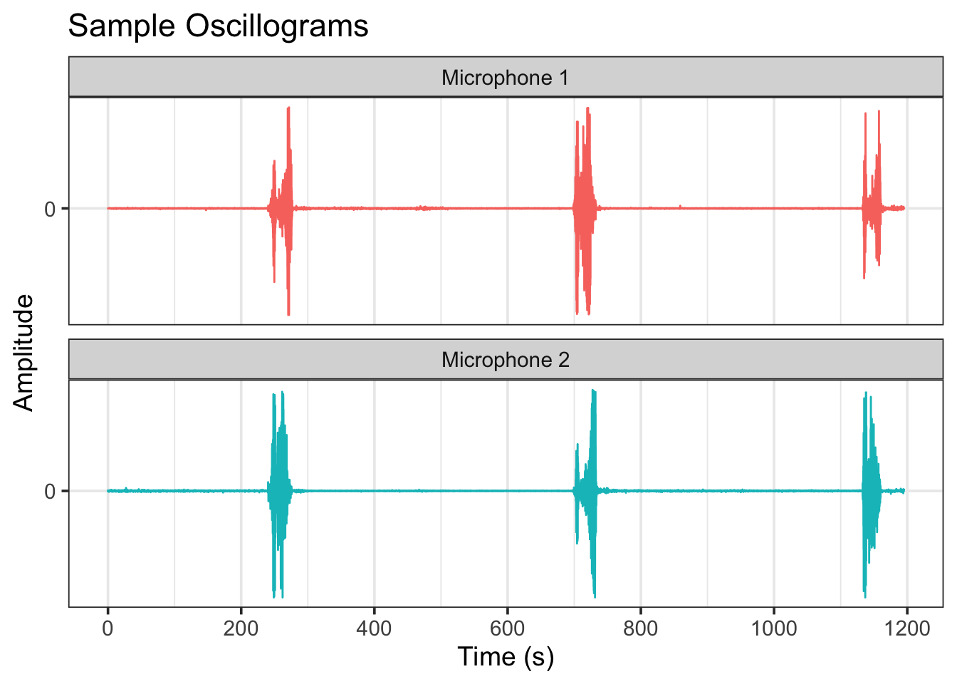

Figure 6: Amplitude oscillograms of simultaneous underwater audio recordings for three wake surf boat passes.

From Figure 6, we see that three boat passes are clearly identified by the recordings. For each boat pass, there are two main peaks. The first peak is from the boat accelerating from a stop, and the second peak is from the boat passing the microphone.

Spectrograms

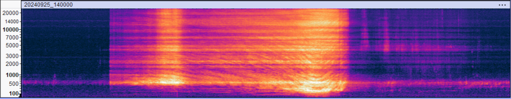
Oscillograms are only one way of “seeing” sound. A more informative (but less intuitive) sound visualization method is the spectrogram. Spectrograms convey the spectral power (essentially the amplitude intensity) of the frequencies that comprise a sound in time, usually with a contour or image plot.

Generally, humans hear sounds from 20 Hz up to 20,000 Hz – above this threshold are the ultrasonic frequencies. For reference, the human voices typically fall between 80 Hz and 250 Hz.

Figure 7 is an Audacity spectrogram of the raw (48 kHz) audio for the first boat pass in Figure 6 as recorded by microphone 1. Note that the frequencies on the y-axis are log-scaled and only go to 24 kHz – half of the sample rate. That’s because the maximum frequency that can be properly resolved (the Nyquist frequency) is half of the sample rate of the instrument (Shannon, 1949). From the spectrogram, we see that the most powerful sound is below 1 kHz. We also see a “U” pattern in the frequency bands from Doppler shift associated with the relative movement of the boat toward, and then away, from the microphone as it passes. Though it wasn’t polished enough to include in this EDA, I am working on a speed estimator using Doppler shift as well.

Figure 7: Spectrogram of the first boat event in Figure 6 as recorded by microphone 1. Brighter colours indicate higher amplitude intensity.

Sound Detection with seewave::timer()

seewave:timer() (Sueur et al., 2008) detects sound ‘events’ in an audio signal above a user-specified amplitude threshold. The audio wave is presented as an “absolute” (i.e., positive) envelope, which simplifies the analysis. I am applying a fairly strong smoothing to the envelope to reduce the number of peaks and choosing a minimum event duration of 15 seconds so that only the ‘big’ sounds are identified. seewave::timer() automatically generates a base R plot for detected events (Figure 8).

# Set up dual panel plot
par(mfrow = c(2, 1))
par(mar = c(5, 4, 2, 2))

t_1 <- seewave::timer(down_1,
             envt = "abs",
             threshold = threshold,
             msmooth = msmooth,
             dmin = dmin,
             plot = TRUE)

t_2 <- seewave::timer(down_2,
             envt = "abs",
             threshold = threshold,
             msmooth = msmooth,
             dmin = dmin,
             plot = TRUE)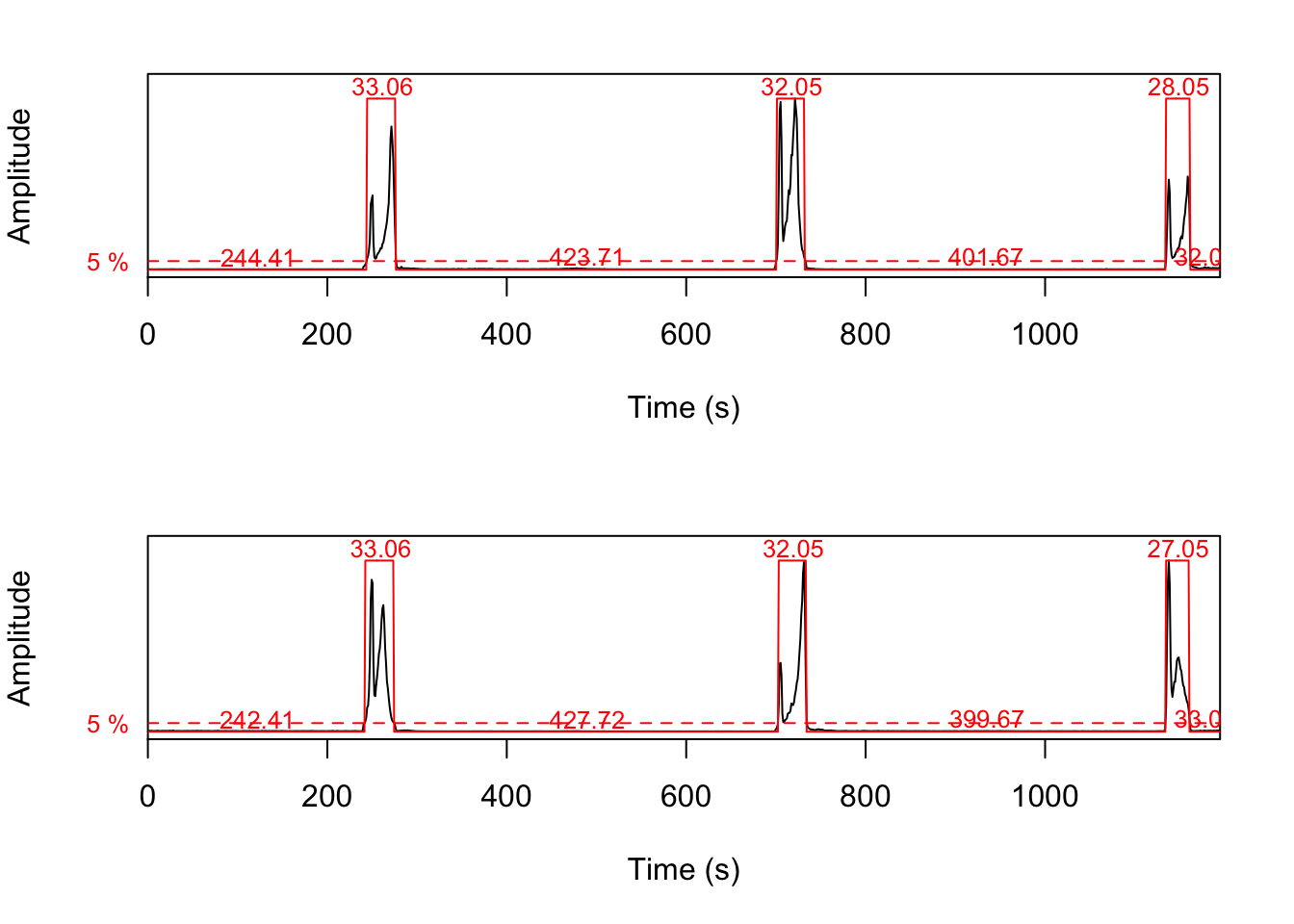

Figure 8: Plots of sound event detection *seewave::timer()* for the sample audio files. Dotted red lines are the 5% minimum amplitude threshold for detection. Red numbers are event (top) and pause (bottom) duration in seconds.

seewave::timer() sound events are used to extract time ranges from the downsampled audio files for peak amplitude identification. The goal is to determine the time stamp of the ‘loudest’ sound in each event. This is done with a for-loop that pulls the event times, scales them back up to the downsampled sample rate, and IDs the local maximums in the downsampled audio signals. Figure 9 shows the seewave::timer() plots, now with the identified peaks overlaid in purple.

Here’s the for-loop code:

# Extract sound event time ranges:
x <- t_1

ranges_1 <- tibble(
  mic = "1",
  event = seq_along(x$s.start),
  start_sec = x$s.start,
  end_sec = x$s.end,
  start_ind = as.integer(trunc(start_sec * down_freq)),
  end_ind = as.integer(trunc(end_sec * down_freq))
)

x <- t_2

ranges_2 <- tibble(
  mic = "2",
  event = seq_along(x$s.start),
  start_sec = x$s.start,
  end_sec = x$s.end,
  start_ind = as.integer(trunc(start_sec * down_freq)),
  end_ind = as.integer(trunc(end_sec * down_freq))
)

# Join into a single tibble
events <- bind_rows(ranges_1, ranges_2)

#### For-loop to identify peak amplitudes ####

# Generate empty list:
peak_list <- vector("list", nrow(events))

# Loop through events data frame:
for (i in seq_len(nrow(events))) {
  
  mic_id <- events$mic[i]
  signal <- signals[[mic_id]]
  
  min <- events$start_ind[i]
  max <- events$end_ind[i]
  
  segment <- signal[min:max]
  
  # Smoothing to match seewave::timer
  env_vec <- as.vector(env(
    wave = segment,
    f = down_freq,
    envt = envt,
    msmooth = msmooth,
    plot = FALSE,
    norm = TRUE
  ))
  
  # Find relative index in the envelope
  peak_ind_rel_env <- which.max(env_vec)
  
  # Scale to segment length
  scale_factor <- length(segment) / length(env_vec)
  peak_ind_rel <- round(peak_ind_rel_env * scale_factor)
  
  # Map to global index
  peak_ind <- peak_ind_rel + min - 1
  peak_sec <- peak_ind / down_freq
  
  # Output
  peak_list[[i]] <- tibble(
    mic = as.character(mic_id),
    event = events$event[i],
    peak_ind = as.integer(peak_ind),
    peak_sec = peak_sec)
}

# Combine results
peaks <- bind_rows(peak_list)

And the plots:

t1_peaks <- peaks |>
  filter(mic == 1) |>
  select(peak_sec) |>
  pull()

t2_peaks <- peaks |>
  filter(mic == 2) |>
  select(peak_sec) |>
  pull()

# Prep double panel base R plot
par(mfrow = c(2, 1))
par(mar = c(5, 4, 2, 2))

# Generate timer() plot again and annotate
seewave::timer(down_1,
               envt = "abs",
               threshold = threshold,
               msmooth = msmooth,
               dmin = dmin,
               plot = TRUE,
               xlab = "")
mtext("Mic 1", adj = 0)
abline(v = t1_peaks, col = "cyan3", lwd = 4, lty = 3)

seewave::timer(down_2,
               envt = "abs",
               threshold = threshold,
               msmooth = msmooth,
               dmin = dmin,
               plot = TRUE)
mtext("Mic 2", adj = 0)
abline(v = t2_peaks, col = "cyan3", lwd = 4, lty = 3)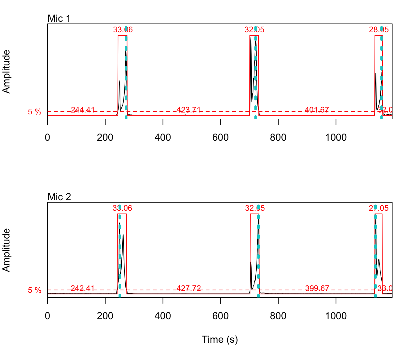

Figure 9: *seewave::timer()* plots with automatically-detected maximum amplitude peaks in as cyan vertical dotted lines.

That looks pretty good! At least for these three events, the loop did it’s job.

Speed Calculation

Now the easy part: calculating speed from these amplitude peaks.

speeds <- peaks |>
  select(mic,
         event,
         peak_sec) |> 
  pivot_wider(names_from = mic,
              values_from = peak_sec,
              names_prefix = "mic_") |> 
  mutate(delta_t = abs(mic_1 - mic_2),
         speed_ms = ifelse(delta_t > 0, dist / delta_t, NA_real_),
         speed_kmh = speed_ms * 3.6)

# Speed table
speeds |>
  mutate(
    across(where(is.numeric), ~ round(.x, 1))
    ) |> 
  kable(
    col.names = c("event", "t_peak_mic_1", "t_peak_mic_2", "delta_t", "speed_ms", "speed_kmh")
    )

Table 4: Sample automatic speed estimates.

event	t_peak_mic_1	t_peak_mic_2	delta_t	speed_ms	speed_kmh
1	272.5	250.4	22	2.9	10.5
2	721.2	731.2	10	6.4	23.1
3	1157.9	1136.9	21	3.1	11.0

And there we go! Three boat speeds estimated from the pair of audio files without any user oversight. The estimated speeds range from 11 to 23 km/h, a bit lower than the true speed (28 km/h), but in the ballpark. For comparison, the manual speed estimates were closer, in the 22 to 28 km/h range.

To get the final “auto_est.csv” results, this process was run across all the pairs of audio files for the three days. It took about 3 minutes. To do this manually took about 6 hours. Ah, the power of automation.

Data Hygiene and Prep

Alright, now that you know how the sausage is made, let’s start working with the results datasets proper.

Manual Results

Not much to do for the manual data, but it can be slightly improved. Removing “#N/A”s that are coercing numeric variables to character and fixing the date.

man <- man |>
  mutate(
    date = as.Date(date, format = "%m/%d/%Y"),
    dist_m = as.numeric(dist_m),
    obs_kmh = as.numeric(obs_kmh),
    pred_kmh = as.numeric(pred_kmh)
    )

head(man)

# A tibble: 6 × 7
  date       time     dist_m pred_kmh obs_kmh type  notes        
  <date>     <time>    <dbl>    <dbl>   <dbl> <chr> <chr>        
1 2024-09-20 14:10:30    100      5.3      10 alum  not our boat?
2 2024-09-20 14:25:09    100      6.6      10 alum  <NA>         
3 2024-09-20 14:34:22    100      5.4      10 alum  not our boat 
4 2024-09-20 14:42:22    100      6.6      10 alum  not out boat 
5 2024-09-20 14:49:58    100     13.5      20 alum  <NA>         
6 2024-09-20 14:59:40    100     10.9      20 alum  not our boat

Ready to roll.

Automated Results

We are going to start with the automatic speed results first – remember Table 3 from way back when? .

I was a bit liberal with all the date and time info. Let’s trim the table down to the essentials and take a peak at the summary:

#  Format date and select desired variables
auto_trim <- auto |>
  mutate(date = as.Date(event_datetime)) |> 
  select(date,
         event_time,
         event,
         mic_1,
         mic_2,
         speed_kmh)

summary(auto_trim)

      date             event_time           event           mic_1         
 Min.   :2024-09-20   Length:145        Min.   : 1.00   Min.   :   1.001  
 1st Qu.:2024-09-20   Class1:hms        1st Qu.:12.00   1st Qu.: 302.506  
 Median :2024-09-25   Class2:difftime   Median :24.00   Median : 623.043  
 Mean   :2024-09-27   Mode  :numeric    Mean   :24.45   Mean   : 620.456  
 3rd Qu.:2024-10-04                     3rd Qu.:35.00   3rd Qu.: 919.538  
 Max.   :2024-10-04                     Max.   :58.00   Max.   :1179.975  
 NA's   :6                              NA's   :6       NA's   :20        
     mic_2           speed_kmh      
 Min.   :  21.03   Min.   :  0.377  
 1st Qu.: 311.52   1st Qu.:  3.225  
 Median : 601.01   Median :  9.876  
 Mean   : 603.87   Mean   : 15.304  
 3rd Qu.: 899.50   3rd Qu.: 19.257  
 Max.   :1193.00   Max.   :123.856  
 NA's   :12        NA's   :27

There are 6 NAs for ‘date’, which occurs when both audio files had no sound events at all. There are 27 NAs for ‘speed_kmh’: the 6 non-event files, but also an additional 21 NAs from when one microphone picked up a sound event but not the other.

Let’s remove the non-event rows and then check that all the times are increasing:

# Filter non-event rows
auto_trim <- auto_trim |> 
  filter(!is.na(date))

# Make sure all times are increasing 
auto_trim |>
  group_by(date) |>
  summarize(times_increasing = all(diff(event_time) > 0))

# A tibble: 3 × 2
  date       times_increasing
  <date>     <lgl>           
1 2024-09-20 TRUE            
2 2024-09-25 FALSE           
3 2024-10-04 TRUE

Whoops, something is out of sequence on Sept 25. Let’s focus in:

auto_trim |>
  group_by(date) |>
  mutate(time_diff_ok = c(TRUE, diff(event_time) > 0)) |>
  filter(!time_diff_ok)

# A tibble: 1 × 7
# Groups:   date [1]
  date       event_time event mic_1 mic_2 speed_kmh time_diff_ok
  <date>     <time>     <dbl> <dbl> <dbl>     <dbl> <lgl>       
1 2024-09-25 14:52:43      19  763.    NA        NA FALSE

Row 19 ‘event_time’ is out of sequence. Upon inspection, this is a quirk of the for-loop logic. A sound event is registered if either mic picks up a sound event. When one mic has a detection, the event_time defaults to that mic’s time index. However, if a sound is picked up by both mics the event_time is calculated as the average between the mic peak times. Thus, it’s possible that an event only detected by one mic could be placed out of sequence based on the averaging of a adjacent event. Something to keep an eye on, but only happened once in these results so probably not serious of a issue.

The next big challenge is matching up the speed estimates with the observations for error analysis. To help facilitate this, I’ll add an estimated direction of navigation (up/down) based which mic picked up the sound even first (mic_1 is upstream of mic_2), and an overall index row for easier referencing.

# Direction
auto_trim <- auto_trim |>
  mutate(est_dir = case_when(
    mic_1 < mic_2 ~ "down",
    mic_1 > mic_2 ~ "up",
    TRUE ~ NA_character_)
  )

# Index
auto_trim <- auto_trim |>
  mutate(index = 1:nrow(auto_trim)) |> 
  relocate(index, .before = date)

auto_trim |> mutate(
  across(where(is.numeric), ~ round(.x, 1))) |>
  kable() |>
  kable_styling(full_width = FALSE) |> 
  scroll_box(height = "400px")

Table 5: Cleaned automatic speed estimate results.

index	date	event_time	event	mic_1	mic_2	speed_kmh	est_dir
1	2024-09-20	14:08:28	1	651.1	366.6	0.8	up
2	2024-09-20	14:10:09	2	NA	609.0	NA	NA
3	2024-09-20	14:25:12	3	292.5	332.6	5.6	down
4	2024-09-20	14:34:25	4	883.5	847.4	6.2	up
5	2024-09-20	14:42:22	5	122.2	163.3	5.4	down
6	2024-09-20	14:49:58	6	607.0	590.0	13.1	up
7	2024-09-20	14:59:41	7	1170.0	1193.0	9.7	down
8	2024-09-20	15:05:25	8	559.9	91.2	0.5	up
9	2024-09-20	15:10:35	9	711.2	558.9	1.5	up
10	2024-09-20	15:12:47	10	845.4	690.2	1.4	up
11	2024-09-20	15:14:34	11	NA	874.5	NA	NA
12	2024-09-20	15:20:47	12	35.1	60.1	8.9	down
13	2024-09-20	15:26:32	13	427.7	357.6	3.2	up
14	2024-09-20	15:26:51	14	NA	411.7	NA	NA
15	2024-09-20	15:41:51	15	104.2	119.2	14.9	down
16	2024-09-20	15:48:53	16	540.9	525.9	14.9	up
17	2024-09-20	15:50:15	17	625.0	605.0	11.2	up
18	2024-09-20	15:58:20	18	1086.8	1114.9	8.0	down
19	2024-09-20	16:03:29	19	389.7	29.0	0.6	up
20	2024-09-20	16:07:58	20	590.0	367.6	1.0	up
21	2024-09-20	16:11:33	21	786.3	601.0	1.2	up
22	2024-09-20	16:15:21	22	1066.8	775.3	0.8	up
23	2024-09-20	16:18:19	23	1122.9	1075.8	4.7	up
24	2024-09-20	16:18:32	24	NA	1112.9	NA	NA
25	2024-09-20	16:21:27	25	85.1	90.2	44.6	down
26	2024-09-20	16:22:15	26	140.2	130.2	22.3	up
27	2024-09-20	16:24:33	27	295.5	251.4	5.1	up
28	2024-09-20	16:25:27	28	348.6	305.5	5.2	up
29	2024-09-20	16:26:22	29	425.7	339.6	2.6	up
30	2024-09-20	16:31:37	30	960.6	434.7	0.4	up
31	2024-09-20	16:32:01	31	NA	721.2	NA	NA
32	2024-09-20	16:35:53	32	NA	953.6	NA	NA
33	2024-09-20	17:12:31	33	741.2	762.3	10.6	down
34	2024-09-20	17:17:57	34	1079.8	1075.8	55.8	up
35	2024-09-20	17:29:00	35	550.9	530.0	10.7	up
36	2024-09-20	17:31:01	36	662.0	660.2	123.9	up
37	2024-09-20	17:34:11	37	835.3	867.6	6.9	down
38	2024-09-20	17:35:16	38	NA	916.7	NA	NA
39	2024-09-25	13:08:46	1	535.9	517.9	13.7	up
40	2024-09-25	13:14:53	2	888.5	899.5	22.4	down
41	2024-09-25	13:18:01	3	1068.8	1093.8	9.9	down
42	2024-09-25	13:23:51	4	238.4	224.4	17.6	up
43	2024-09-25	13:30:03	5	598.0	609.0	22.4	down
44	2024-09-25	13:37:08	6	1037.7	1018.7	13.0	up
45	2024-09-25	13:43:55	7	229.4	242.4	19.0	down
46	2024-09-25	13:51:41	8	708.2	694.2	17.6	up
47	2024-09-25	13:56:58	9	936.6	1100.8	1.5	down
48	2024-09-25	13:58:07	10	1087.8	NA	NA	NA
49	2024-09-25	14:04:21	11	272.5	250.4	11.2	up
50	2024-09-25	14:12:06	12	721.2	731.2	24.7	down
51	2024-09-25	14:19:07	13	1157.9	1136.9	11.8	up
52	2024-09-25	14:25:07	14	302.5	311.5	27.4	down
53	2024-09-25	14:29:52	15	606.0	579.0	9.1	up
54	2024-09-25	14:33:44	16	820.4	829.4	27.4	down
55	2024-09-25	14:47:33	17	144.2	763.3	0.4	down
56	2024-09-25	14:54:06	18	518.9	1175.0	0.4	down
57	2024-09-25	14:52:43	19	763.3	NA	NA	NA
58	2024-09-25	14:59:26	20	1167.0	NA	NA	NA
59	2024-09-25	15:06:47	21	444.7	370.6	3.3	up
60	2024-09-25	15:12:41	22	749.3	774.3	9.9	down
61	2024-09-25	15:18:58	23	1150.9	1125.9	9.9	up
62	2024-09-25	15:24:21	24	234.4	289.5	4.5	down
63	2024-09-25	15:33:31	25	821.4	802.3	13.0	up
64	2024-09-25	15:39:39	26	1180.0	1180.0	NA	NA
65	2024-09-25	15:40:11	27	1.0	21.0	12.3	down
66	2024-09-25	15:47:28	28	474.8	422.7	4.7	up
67	2024-09-25	15:54:43	29	834.4	933.6	2.5	down
68	2024-09-25	15:55:19	30	919.5	NA	NA	NA
69	2024-09-25	16:02:30	31	157.3	143.2	17.6	up
70	2024-09-25	16:08:57	32	530.9	544.9	17.6	down
71	2024-09-25	16:15:35	33	945.6	925.5	12.3	up
72	2024-09-25	16:22:01	34	109.2	133.2	10.3	down
73	2024-09-25	16:28:30	35	514.9	505.8	27.4	up
74	2024-09-25	16:34:54	36	890.5	899.5	27.4	down
75	2024-09-25	16:37:40	37	1063.8	1057.8	41.2	up
76	2024-09-25	16:43:10	38	188.3	193.3	49.4	down
77	2024-09-25	16:48:08	39	NA	488.8	NA	NA
78	2024-09-25	17:15:31	40	995.7	867.5	1.9	up
79	2024-09-25	17:24:37	41	175.3	380.6	1.2	down
80	2024-09-25	17:26:26	42	386.6	NA	NA	NA
81	2024-09-25	17:47:48	43	509.3	427.3	3.0	up
82	2024-10-04	12:08:16	1	529.9	463.8	3.5	up
83	2024-10-04	12:11:13	2	660.1	686.1	8.9	down
84	2024-10-04	12:20:54	3	27.0	81.1	4.3	down
85	2024-10-04	12:33:19	4	816.4	783.3	7.0	up
86	2024-10-04	12:38:22	5	1023.7	1181.0	1.5	down
87	2024-10-04	12:39:35	6	1176.0	NA	NA	NA
88	2024-10-04	12:40:31	7	19.0	44.1	9.2	down
89	2024-10-04	12:44:23	8	297.5	230.4	3.4	up
90	2024-10-04	12:45:38	9	392.7	283.5	2.1	up
91	2024-10-04	12:48:27	10	647.1	367.6	0.8	up
92	2024-10-04	12:52:54	11	960.6	588.0	0.6	up
93	2024-10-04	12:57:43	12	1135.9	991.7	1.6	up
94	2024-10-04	12:58:43	13	NA	1123.9	NA	NA
95	2024-10-04	13:03:26	14	195.3	218.4	10.0	down
96	2024-10-04	13:09:42	15	589.0	577.0	19.3	up
97	2024-10-04	13:15:32	16	926.5	938.6	19.3	down
98	2024-10-04	13:23:28	17	213.4	203.3	23.1	up
99	2024-10-04	13:30:29	18	626.0	632.1	38.5	down
100	2024-10-04	13:33:48	19	NA	828.4	NA	NA
101	2024-10-04	13:40:26	20	28.0	24.0	57.8	up
102	2024-10-04	13:53:24	21	802.3	806.3	57.8	down
103	2024-10-04	13:55:12	22	920.5	903.5	13.6	up
104	2024-10-04	14:00:56	23	66.1	47.1	12.2	up
105	2024-10-04	14:06:03	24	357.6	368.6	21.0	down
106	2024-10-04	14:13:17	25	803.3	792.3	21.0	up
107	2024-10-04	14:19:27	26	1166.0	1170.0	57.8	down
108	2024-10-04	14:24:55	27	297.5	293.5	57.8	up
109	2024-10-04	14:32:22	28	726.2	759.3	7.0	down
110	2024-10-04	14:38:00	29	1087.8	1072.8	15.4	up
111	2024-10-04	14:43:50	30	226.4	234.4	28.9	down
112	2024-10-04	14:46:23	31	378.6	388.6	23.1	down
113	2024-10-04	14:52:07	32	732.2	723.2	25.7	up
114	2024-10-04	14:56:51	33	1009.7	1013.7	57.8	down
115	2024-10-04	15:03:04	34	186.3	182.3	57.8	up
116	2024-10-04	15:14:38	35	877.5	880.5	77.0	down
117	2024-10-04	15:29:04	36	562.9	526.9	6.4	up
118	2024-10-04	15:33:04	37	794.3	775.3	12.2	up
119	2024-10-04	15:36:50	38	1034.7	985.6	4.7	up
120	2024-10-04	15:37:34	39	NA	1054.8	NA	NA
121	2024-10-04	15:42:59	40	186.3	172.3	16.5	up
122	2024-10-04	15:48:40	41	514.9	525.9	21.0	down
123	2024-10-04	15:55:10	42	923.5	897.5	8.9	up
124	2024-10-04	16:01:13	43	87.1	60.1	8.6	up
125	2024-10-04	16:03:44	44	346.6	103.2	1.0	up
126	2024-10-04	16:07:54	45	623.0	326.5	0.8	up
127	2024-10-04	16:12:49	46	913.5	626.0	0.8	up
128	2024-10-04	16:15:05	47	NA	905.5	NA	NA
129	2024-10-04	16:20:48	48	36.1	61.1	9.2	down
130	2024-10-04	16:24:56	49	277.5	315.5	6.1	down
131	2024-10-04	16:27:30	50	456.8	444.7	19.3	up
132	2024-10-04	16:30:03	51	617.0	590.0	8.6	up
133	2024-10-04	16:35:59	52	948.6	969.6	11.0	down
134	2024-10-04	16:39:39	53	NA	1180.0	NA	NA
135	2024-10-04	16:46:53	54	605.0	221.4	0.6	up
136	2024-10-04	16:51:45	55	795.3	615.0	1.3	up
137	2024-10-04	16:55:01	56	999.7	802.3	1.2	up
138	2024-10-04	16:57:31	57	1107.9	995.7	2.1	up
139	2024-10-04	16:58:20	58	NA	1100.8	NA	NA

I’m happy with how this is looking. Let’s move to the observational data.

Observational Data

head(obs)

# A tibble: 6 × 11
      date event time_NDA time_SR boat_dist_m speed_kmh dir   boat_type shaper
     <dbl> <dbl> <time>   <time>        <dbl> <chr>     <chr> <chr>     <chr> 
1 20240920     1 14:09:00    NA           100 10        up    alum      <NA>  
2 20240920     2 14:24:31    NA           100 10        down  alum      <NA>  
3 20240920     3 14:34:12    NA           100 10        up    alum      <NA>  
4 20240920     4 14:42:20    NA           100 10        down  alum      <NA>  
5 20240920     5 14:49:55    NA           100 20        up    alum      <NA>  
6 20240920     6 14:59:35    NA           100 20        down  alum      <NA>  
# ℹ 2 more variables: mic_dist_m <dbl>, notes <chr>

Let’s make ‘date’ a date class.

obs <- obs |>
  mutate(date = ymd(date)) |> 
  arrange(date)

Speed is also in character class. Let’s check for non-numerics with some regex.

# Look for non-digits
obs |> 
  filter(!str_detect(speed_kmh, "\\d")) |> 
  select(speed_kmh) |> 
  pull()

 [1] "S" "S" "S" "M" "M" "S" "F" "M" "S" "S" "F" "F" "S"

Right, there were some civilian boat passes interspersed in the trials. I sometimes added a qualitative speed (S = slow, M = medium, F = fast) for those. This is coercing the the speed_kmh variable to character. Lets split the speed column in two, one for numeric, one for character.

obs <- obs |>
  mutate(
    speed_kmh_num = as.numeric(speed_kmh),
    speed_qual = if_else(is.na(speed_kmh_num), speed_kmh, NA_character_),
    speed_kmh = speed_kmh_num
  ) |> 
  select(-speed_kmh_num) |> 
  relocate(speed_qual, .after = speed_kmh)

There are two time columns of boat pass times, one for each observer. Times are generally close, but have some variability. I’ll leave both in for now, as I’m not sure which observer was doing a better job!

Are all the event times increasing?

obs |>
  group_by(date) |>
  summarize(across(c(time_NDA, time_SR), ~ all(diff(.x) > 0)))

# A tibble: 4 × 3
  date       time_NDA time_SR
  <date>     <lgl>    <lgl>  
1 2024-09-20 TRUE     NA     
2 2024-09-25 TRUE     TRUE   
3 2024-10-04 NA       TRUE   
4 2024-10-09 NA       TRUE

All the time events are in order. However, we see that duplicate time observations are only available for Sept 25, and that there is an extra date included in the observations. We are only validating for the three days, so Oct 9 can be removed.

obs <- obs |> 
  filter(!date == "2024-10-09")

Finally, lets add an index to number all observations sequentially.

obs <- obs |> 
  mutate(index = 1:nrow(obs)) |> 
  relocate(index, .before = event)

obs |> mutate(
  across(where(is.numeric), ~ round(.x, 1))) |>
  kable() |>
  kable_styling(full_width = FALSE) |> 
  scroll_box(height = "400px")

Table 6: Cleaned observational data.

date	index	event	time_NDA	time_SR	boat_dist_m	speed_kmh	speed_qual	dir	boat_type	shaper	mic_dist_m	notes
2024-09-20	1	1	14:09:00	NA	100	10.0	NA	up	alum	NA	62.1	NA
2024-09-20	2	2	14:24:31	NA	100	10.0	NA	down	alum	NA	62.1	NA
2024-09-20	3	3	14:34:12	NA	100	10.0	NA	up	alum	NA	62.1	NA
2024-09-20	4	4	14:42:20	NA	100	10.0	NA	down	alum	NA	62.1	NA
2024-09-20	5	5	14:49:55	NA	100	20.0	NA	up	alum	NA	62.1	NA
2024-09-20	6	6	14:59:35	NA	100	20.0	NA	down	alum	NA	62.1	NA
2024-09-20	7	7	15:11:35	NA	100	17.0	NA	up	alum	NA	62.1	NA
2024-09-20	8	8	15:14:00	NA	NA	NA	NA	NA	NA	NA	62.1	not our boat
2024-09-20	9	9	15:20:44	NA	100	21.0	NA	down	alum	NA	62.1	NA
2024-09-20	10	10	15:26:55	NA	100	30.0	NA	up	alum	NA	62.1	NA
2024-09-20	11	11	15:41:50	NA	100	27.0	NA	down	alum	NA	62.1	NA
2024-09-20	12	12	15:48:48	NA	100	28.0	NA	up	alum	NA	62.1	NA
2024-09-20	13	13	15:50:34	NA	NA	NA	NA	NA	NA	NA	62.1	not our boat
2024-09-20	14	14	15:58:15	NA	60	10.0	NA	down	alum	NA	62.1	NA
2024-09-20	15	15	16:06:08	NA	60	10.0	NA	up	alum	NA	62.1	NA
2024-09-20	16	16	16:09:55	NA	NA	NA	NA	NA	NA	NA	62.1	not our boat
2024-09-25	17	1	12:48:39	12:49:00	100	6.0	NA	up	wake	off	68.7	no wake
2024-09-25	18	2	12:53:22	12:53:20	100	6.0	NA	down	wake	off	68.7	no wake
2024-09-25	19	3	12:56:30	12:56:50	60	5.5	NA	up	wake	off	68.7	NA
2024-09-25	20	4	12:59:00	12:59:10	60	6.0	NA	down	wake	off	68.7	NA
2024-09-25	21	5	13:02:44	13:02:45	30	6.0	NA	up	wake	off	68.7	NA
2024-09-25	22	6	13:05:08	13:05:20	30	6.0	NA	down	wake	off	68.7	NA
2024-09-25	23	7	13:08:48	13:08:50	100	27.0	NA	up	wake	off	68.7	NA
2024-09-25	24	8	13:15:07	13:14:55	100	27.0	NA	down	wake	off	68.7	NA
2024-09-25	25	9	13:18:23	13:18:10	NA	NA	S	down	cruiser	NA	68.7	not our boat
2024-09-25	26	10	13:23:40	13:23:50	100	18.0	NA	up	wake	on	68.7	NA
2024-09-25	27	11	13:30:12	13:30:12	100	18.0	NA	down	wake	on	68.7	NA
2024-09-25	28	12	13:36:59	13:36:59	60	18.0	NA	up	wake	on	68.7	NA
2024-09-25	29	13	13:43:45	13:43:45	60	18.0	NA	down	wake	on	68.7	NA
2024-09-25	30	14	13:51:34	13:51:34	30	18.0	NA	up	wake	on	68.7	NA
2024-09-25	31	15	13:58:07	13:57:07	30	18.0	NA	down	wake	on	68.7	NA
2024-09-25	32	16	14:04:26	14:04:20	30	27.0	NA	up	wake	on	68.7	NA
2024-09-25	33	17	14:12:02	14:12:02	30	27.0	NA	down	wake	on	68.7	NA
2024-09-25	34	18	14:19:12	14:19:12	60	27.0	NA	up	wake	on	68.7	NA
2024-09-25	35	19	14:24:59	14:24:59	60	27.0	NA	down	wake	on	68.7	NA
2024-09-25	36	20	14:29:45	14:29:45	60	27.0	NA	up	wake	on	68.7	NA
2024-09-25	37	21	14:33:39	14:33:39	60	27.0	NA	down	wake	on	68.7	NA
2024-09-25	38	22	14:41:56	14:42:00	100	10.0	NA	up	wake	on	68.7	NA
2024-09-25	39	23	14:48:40	14:48:45	100	10.0	NA	down	wake	on	68.7	NA
2024-09-25	40	24	14:52:55	14:52:55	100	27.0	NA	up	wake	on	68.7	NA
2024-09-25	41	25	14:59:24	14:59:28	100	27.0	NA	down	wake	on	68.7	NA
2024-09-25	42	26	15:07:05	15:07:05	60	10.0	NA	up	wake	on	68.7	NA
2024-09-25	43	27	15:12:34	15:12:34	60	10.0	NA	down	wake	on	68.7	NA
2024-09-25	44	28	15:18:52	15:18:57	30	10.0	NA	up	wake	on	68.7	NA
2024-09-25	45	29	15:24:32	15:24:40	30	10.0	NA	down	wake	on	68.7	NA
2024-09-25	46	30	15:33:21	15:33:21	100	18.0	NA	up	wake	off	68.7	NA
2024-09-25	47	31	15:40:09	15:40:09	100	18.0	NA	down	wake	off	68.7	NA
2024-09-25	48	32	15:47:43	15:47:43	60	18.0	NA	up	wake	off	68.7	NA
2024-09-25	49	33	15:55:21	15:55:21	60	18.0	NA	down	wake	off	68.7	NA
2024-09-25	50	34	16:02:25	16:02:25	30	18.0	NA	up	wake	off	68.7	NA
2024-09-25	51	35	16:08:53	16:08:10	30	18.0	NA	down	wake	off	68.7	RBR tipped
2024-09-25	52	36	16:15:35	16:15:35	60	27.0	NA	up	wake	off	68.7	NA
2024-09-25	53	37	16:22:03	16:22:03	60	27.0	NA	down	wake	off	68.7	NA
2024-09-25	54	38	16:28:28	16:28:28	30	27.0	NA	up	wake	off	68.7	NA
2024-09-25	55	39	16:34:51	16:34:51	30	27.0	NA	down	wake	off	68.7	NA
2024-09-25	56	40	16:37:17	16:37:17	65	55.0	NA	up	wake	off	68.7	NA
2024-09-25	57	41	16:43:00	16:43:20	30	57.0	NA	down	wake	off	68.7	NA
2024-10-04	58	1	NA	11:58:30	65	NA	S	up	cruiser	NA	64.3	not our boat
2024-10-04	59	2	NA	12:08:40	100	9.7	NA	up	cruiser	NA	64.3	NA
2024-10-04	60	3	NA	12:11:15	65	NA	S	down	cruiser	NA	64.3	not our boat
2024-10-04	61	4	NA	12:20:30	100	9.9	NA	down	cruiser	NA	64.3	NA
2024-10-04	62	5	NA	12:33:20	60	9.7	NA	up	cruiser	NA	64.3	NA
2024-10-04	63	6	NA	12:40:27	60	9.7	NA	down	cruiser	NA	64.3	NA
2024-10-04	64	7	NA	12:44:55	50	NA	M	up	runabout	NA	64.3	not our boat
2024-10-04	65	8	NA	12:46:25	80	NA	M	up	pontoon	NA	64.3	not our boat
2024-10-04	66	9	NA	12:50:40	30	9.5	NA	up	cruiser	NA	64.3	NA
2024-10-04	67	10	NA	12:56:15	40	NA	S	down	runabout	NA	64.3	not our boat
2024-10-04	68	11	NA	12:58:51	95	NA	F	up	ski	NA	64.3	not our boat
2024-10-04	69	12	NA	13:03:16	30	9.3	NA	down	cruiser	NA	64.3	NA
2024-10-04	70	13	NA	13:09:48	30	21.7	NA	up	cruiser	NA	64.3	Big!
2024-10-04	71	14	NA	13:15:29	30	20.1	NA	down	cruiser	NA	64.3	Big!
2024-10-04	72	15	NA	13:23:24	30	32.1	NA	up	cruiser	NA	64.3	NA
2024-10-04	73	16	NA	13:30:26	30	30.9	NA	down	cruiser	NA	64.3	NA
2024-10-04	74	17	NA	13:40:35	30	48.2	NA	up	cruiser	NA	64.3	NA
2024-10-04	75	18	NA	13:53:23	30	50.7	NA	down	cruiser	NA	64.3	NA
2024-10-04	76	19	NA	13:55:10	85	NA	M	up	alum	NA	64.3	not our boat
2024-10-04	77	20	NA	14:00:57	60	27.8	NA	up	cruiser	NA	64.3	NA
2024-10-04	78	21	NA	14:06:00	60	21.5	NA	down	cruiser	NA	64.3	NA
2024-10-04	79	22	NA	14:13:10	60	21.6	NA	up	cruiser	NA	64.3	NA
2024-10-04	80	23	NA	14:19:28	60	60.0	NA	down	cruiser	NA	64.3	NA
2024-10-04	81	24	NA	14:24:51	60	59.5	NA	up	cruiser	NA	64.3	NA
2024-10-04	82	25	NA	14:32:15	100	19.7	NA	down	cruiser	NA	64.3	NA
2024-10-04	83	26	NA	14:38:06	100	19.9	NA	up	cruiser	NA	64.3	NA
2024-10-04	84	27	NA	14:43:46	100	59.5	NA	down	cruiser	NA	64.3	NA
2024-10-04	85	28	NA	14:46:24	65	NA	NA	down	alum	NA	64.3	not our boat
2024-10-04	86	29	NA	14:52:18	100	62.1	NA	up	cruiser	NA	64.3	NA
2024-10-04	87	30	NA	14:56:50	60	61.7	NA	down	cruiser	NA	64.3	NA
2024-10-04	88	31	NA	15:03:03	30	61.1	NA	up	cruiser	NA	64.3	NA
2024-10-04	89	32	NA	15:11:12	60	NA	NA	down	ski	NA	64.3	not our boat
2024-10-04	90	33	NA	15:14:38	30	67.8	NA	down	cruiser	NA	64.3	NA
2024-10-04	91	34	NA	15:29:05	50	NA	S	up	runabout	NA	64.3	not our boat
2024-10-04	92	35	NA	15:33:00	30	11.2	NA	up	cruiser	NA	64.3	NA
2024-10-04	93	36	NA	15:37:21	30	11.5	NA	down	cruiser	NA	64.3	NA
2024-10-04	94	37	NA	15:43:00	30	18.6	NA	up	cruiser	NA	64.3	NA
2024-10-04	95	38	NA	15:48:43	30	23.1	NA	down	cruiser	NA	64.3	NA
2024-10-04	96	39	NA	15:55:13	60	11.6	NA	up	cruiser	NA	64.3	NA
2024-10-04	97	40	NA	16:01:35	60	11.6	NA	down	cruiser	NA	64.3	NA
2024-10-04	98	41	NA	16:05:37	60	22.0	NA	up	cruiser	NA	64.3	NA
2024-10-04	99	42	NA	16:10:24	100	64.1	NA	down	cruiser	NA	64.3	NA
2024-10-04	100	43	NA	16:15:10	100	67.1	NA	up	cruiser	NA	64.3	NA
2024-10-04	101	44	NA	16:20:50	100	22.0	NA	down	cruiser	NA	64.3	NA
2024-10-04	102	45	NA	16:24:48	35	NA	S	down	runabout	NA	64.3	not our boat
2024-10-04	103	46	NA	16:30:05	100	20.9	NA	up	cruiser	NA	64.3	NA
2024-10-04	104	47	NA	16:36:31	100	10.5	NA	down	cruiser	NA	64.3	NA
2024-10-04	105	48	NA	16:44:21	100	10.7	NA	up	cruiser	NA	64.3	NA
2024-10-04	106	49	NA	16:50:10	60	23.9	NA	down	runabout	NA	64.3	NA
2024-10-04	107	50	NA	16:53:22	60	NA	F	down	cruiser	NA	64.3	knee boarder
2024-10-04	108	51	NA	16:56:36	60	59.9	NA	up	cruiser	NA	64.3	NA
2024-10-04	109	52	NA	16:58:25	60	NA	F	up	runabout	NA	64.3	not our boat

Data Exploration

Now what do these numbers tell us?

Automated Estimates

How many sound events were detected by the mics?

nrow(auto_trim)

[1] 139

How many events yielded a speed estimate?

sum(!is.na(auto_trim$speed_kmh))

[1] 118

What percentage of detected sound events don’t have a speed estimate?

auto_trim |> 
  filter(is.na(speed_kmh)) |> 
  summarize("NAs" = n(), "%" = round((NAs / nrow(auto_trim) * 100), 1))

# A tibble: 1 × 2
    NAs   `%`
  <int> <dbl>
1    21  15.1

Which mic picked up the most events?

auto_trim |>
  summarize(across(c(mic_1 , mic_2), ~ sum(!is.na(.x))))

# A tibble: 1 × 2
  mic_1 mic_2
  <int> <int>
1   125   133

Mic 2 (downstream) is the winner. Perhaps this is a feature of slightly different positioning or bathymetry.

Let’s take a quick look at the distribution of automatically generated speed estimates.

auto_trim |>
  filter(!is.na(speed_kmh)) |> 
  ggplot(aes(x = speed_kmh)) +
  geom_histogram(binwidth = 1, col = "pink") +
  labs(title = "Automated",
       x = "Speed (km/h)",
       y = "Count") +
  theme_bw(base_size = 14)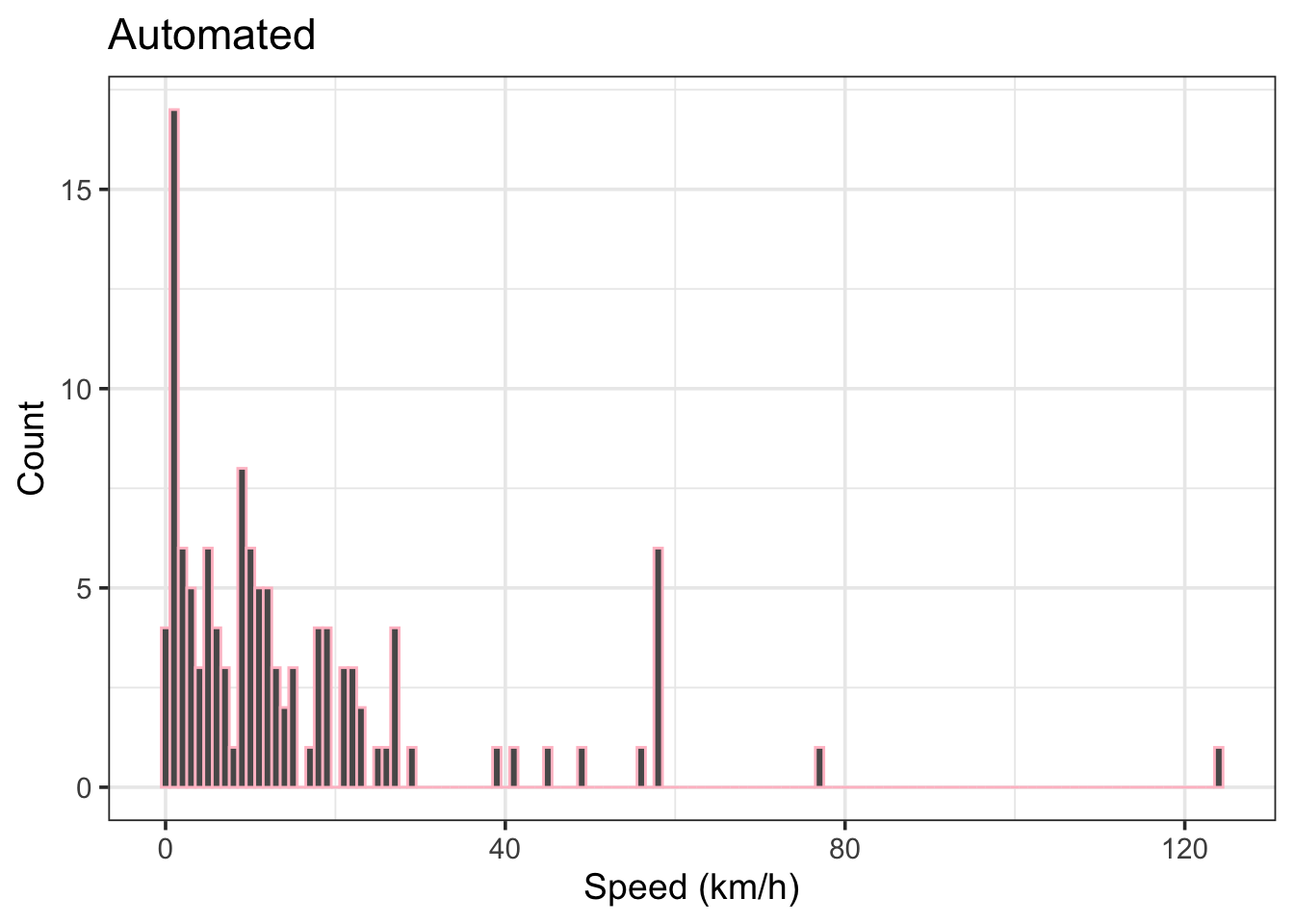

Figure 10: Histogram of automatic speed estimates (km/h).

In Figure 10, there are a lot of estimates < 1 km/h which are probably not legitimate. It also looks like there is a very high speed estimate around 125 km/h.

auto_trim |> 
  select(speed_kmh) |> 
  slice_max(speed_kmh, n = 5) |> 
  round(1)

# A tibble: 5 × 1
  speed_kmh
      <dbl>
1     124. 
2      77  
3      57.8
4      57.8
5      57.8

Yep, 124 km/h boat speed is not impossible, but nearly double the actual speed ranges tested in these trials. But, because this is a method validation, need to leave this in the results.

Observations

How many actual boat passes were observed? This includes the control boats and any civilian boats that came through during the trials.

nrow(obs)

[1] 109

And of these 109 boat passes, how many were by the research team?

sum(!is.na(obs$speed_kmh))

[1] 92

We have 92 control passes to compare to the estimated results.

And the observational speed distribution:

obs |>
  filter(!is.na(speed_kmh)) |> 
  ggplot(aes(x = speed_kmh)) +
  geom_histogram(binwidth = 1, col = "pink") +
  labs(title = "Observed",
       x = "Speed (km/h)",
       y = "Count") +
  theme_bw(base_size = 14)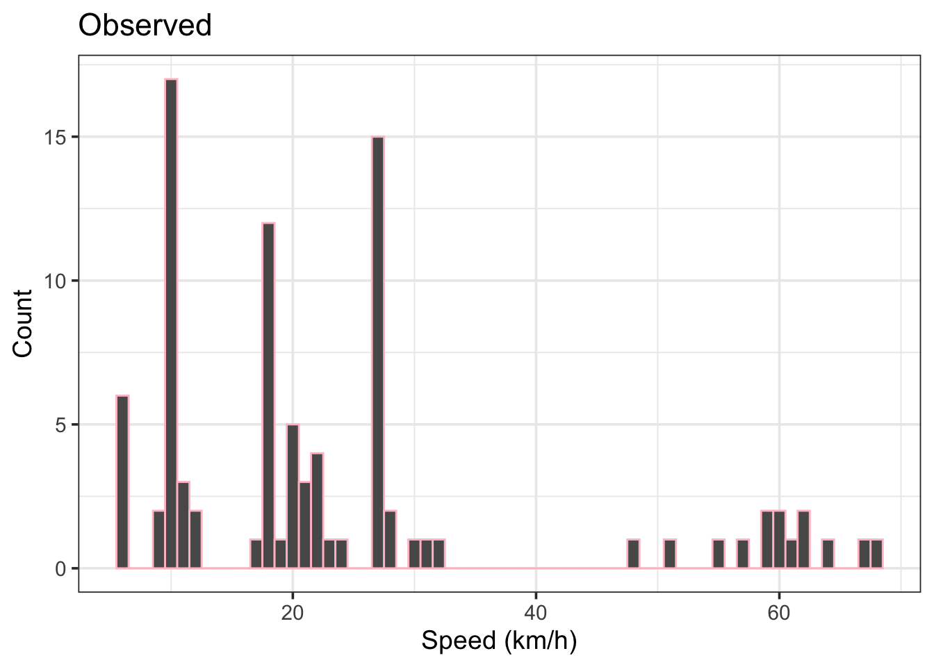

Figure 11: Histogram of observed speeds (km/h).

Figure 11 looks good. There is a trimodality in the distribution corresponding to slow (~ 10 km/h), medium (15 to 30 km/h), and fast (> 45 to 70 km/h) speed ranges of the trials. There are far fewer very slow speeds (< 5 km/h) compared to the automatic estimates.

obs |>
  filter(!is.na(speed_kmh)) |>
  mutate(speed_kmh = round(speed_kmh, digits = 0)) |> 
  count(speed_kmh, sort = TRUE) |> 
  head(n = 5)

# A tibble: 5 × 2
  speed_kmh     n
      <dbl> <int>
1        10    18
2        27    15
3        18    12
4         6     6
5        20     5

Speeds of 10, 27, and 18 km/h were most common in controlled trials.

Matching Auto-Generated Speeds to Observations

There are 92 benchmark observations to compare to the 118 auto-identified speed estimates. But how do we know which events to compare? To do this, it’s necessary to match observed passes to the estimate events - which may be difficult to do automatically. Let’s see what we can do.

We’ll filter both the auto and observed results to remove rows without speed values.

auto_trim <- auto_trim |> 
  filter(!is.na(speed_kmh))

obs <- obs |> 
  filter(!is.na(speed_kmh))

I’m going to simplify the double observation times for Sept 25 by averaging into a single column.

obs <- obs |>
  mutate(
    obs_time = case_when(
      !is.na(time_NDA) & !is.na(time_SR) ~ (time_NDA + time_SR) / 2,
      !is.na(time_NDA) & is.na(time_SR) ~ time_NDA,
      is.na(time_NDA) & !is.na(time_SR) ~ time_SR),
    time_NDA = NULL,
    time_SR = NULL
  ) |> 
  relocate(obs_time, .after =  event)

Now some heavy lifting. Building up a greedy for-loop that will look for the closest time match between actual boat pass events and the auto-generated speed events. If the closest actual event is separated by more than 30 seconds from the auto-event, a penalty is applied that reduces the likelihood of the events being matched. The loop will also check if the estiamted direction of travel matches observation.

# Set time window (in seconds)
t_max <- 30

# Create all valid matches within time threshold
match_candidates <- inner_join(
  auto_trim |>
    select(auto_index = index,
           date,
           auto_time = event_time,
           auto_speed_kmh = speed_kmh,
           est_dir),
  obs |>
    select(obs_index = index,
           date,
           obs_time,
           obs_speed_kmh = speed_kmh,
           obs_dir = dir),
  by = "date",
  relationship = "many-to-many"
) |>
  mutate(
    time_diff = abs(as.numeric(difftime(auto_time, obs_time, units = "secs"))),
    dir_penalty = if_else(est_dir != obs_dir, 15, 0),
    match_score = time_diff + dir_penalty
  ) |>
  filter(time_diff <= t_max) |>
  arrange(match_score)

# Greedy loop to assign best unique matches
used_auto <- c()
used_obs <- c()
final_matches <- list()

for (i in seq_len(nrow(match_candidates))) {
  row <- match_candidates[i, ]
  
  if (!(row$auto_index %in% used_auto) && !(row$obs_index %in% used_obs)) {
    final_matches[[length(final_matches) + 1]] <- row
    used_auto <- c(used_auto, row$auto_index)
    used_obs <- c(used_obs, row$obs_index)
  }
}

# Final formatting
matched <- bind_rows(final_matches) |>
  mutate(
    dir_match = case_when(
      obs_dir != est_dir ~ "no",
      TRUE ~ "yes"
    ),
    obs_dir = obs_dir,
    speed_diff = auto_speed_kmh - obs_speed_kmh,
    abs_speed_diff = abs(speed_diff)
  ) |>
  select(
    obs_index,
    auto_index,
    date,
    obs_time,
    auto_time,
    time_diff,
    obs_dir,
    dir_match,
    obs_speed_kmh,
    auto_speed_kmh,
    speed_diff,
    abs_speed_diff
  ) |>
  arrange(date, auto_time)

matched |>
  mutate(across(where(is.numeric), ~ round(.x, 1))) |>
  kable() |>
  kable_styling(full_width = FALSE) |> 
  scroll_box(height = "400px")

Table 7: Results of greedy loop to match observations to auto-generated speed estimates.

obs_index	auto_index	date	obs_time	auto_time	time_diff	obs_dir	dir_match	obs_speed_kmh	auto_speed_kmh	speed_diff	abs_speed_diff
3	4	2024-09-20	14:34:12.0	14:34:25	13.0	up	yes	10.0	6.2	-3.8	3.8
4	5	2024-09-20	14:42:20.0	14:42:22	2.0	down	yes	10.0	5.4	-4.6	4.6
5	6	2024-09-20	14:49:55.0	14:49:58	3.0	up	yes	20.0	13.1	-6.9	6.9
6	7	2024-09-20	14:59:35.0	14:59:41	6.0	down	yes	20.0	9.7	-10.3	10.3
9	12	2024-09-20	15:20:44.0	15:20:47	3.0	down	yes	21.0	8.9	-12.1	12.1
10	13	2024-09-20	15:26:55.0	15:26:32	23.0	up	yes	30.0	3.2	-26.8	26.8
11	15	2024-09-20	15:41:50.0	15:41:51	1.0	down	yes	27.0	14.9	-12.1	12.1
12	16	2024-09-20	15:48:48.0	15:48:53	5.0	up	yes	28.0	14.9	-13.1	13.1
14	18	2024-09-20	15:58:15.0	15:58:20	5.0	down	yes	10.0	8.0	-2.0	2.0
23	39	2024-09-25	13:08:49.0	13:08:46	3.0	up	yes	27.0	13.7	-13.3	13.3
24	40	2024-09-25	13:15:01.0	13:14:53	8.0	down	yes	27.0	22.4	-4.6	4.6
26	42	2024-09-25	13:23:45.0	13:23:51	6.0	up	yes	18.0	17.6	-0.4	0.4
27	43	2024-09-25	13:30:12.0	13:30:03	9.0	down	yes	18.0	22.4	4.4	4.4
28	44	2024-09-25	13:36:59.0	13:37:08	9.0	up	yes	18.0	13.0	-5.0	5.0
29	45	2024-09-25	13:43:45.0	13:43:55	10.0	down	yes	18.0	19.0	1.0	1.0
30	46	2024-09-25	13:51:34.0	13:51:41	7.0	up	yes	18.0	17.6	-0.4	0.4
32	49	2024-09-25	14:04:23.0	14:04:21	2.0	up	yes	27.0	11.2	-15.8	15.8
33	50	2024-09-25	14:12:02.0	14:12:06	4.0	down	yes	27.0	24.7	-2.3	2.3
34	51	2024-09-25	14:19:12.0	14:19:07	5.0	up	yes	27.0	11.8	-15.2	15.2
35	52	2024-09-25	14:24:59.0	14:25:07	8.0	down	yes	27.0	27.4	0.4	0.4
36	53	2024-09-25	14:29:45.0	14:29:52	7.0	up	yes	27.0	9.1	-17.9	17.9
37	54	2024-09-25	14:33:39.0	14:33:44	5.0	down	yes	27.0	27.4	0.4	0.4
42	59	2024-09-25	15:07:05.0	15:06:47	18.0	up	yes	10.0	3.3	-6.7	6.7
43	60	2024-09-25	15:12:34.0	15:12:41	7.0	down	yes	10.0	9.9	-0.1	0.1
44	61	2024-09-25	15:18:54.5	15:18:58	3.5	up	yes	10.0	9.9	-0.1	0.1
45	62	2024-09-25	15:24:36.0	15:24:21	15.0	down	yes	10.0	4.5	-5.5	5.5
46	63	2024-09-25	15:33:21.0	15:33:31	10.0	up	yes	18.0	13.0	-5.0	5.0
47	65	2024-09-25	15:40:09.0	15:40:11	2.0	down	yes	18.0	12.3	-5.7	5.7
48	66	2024-09-25	15:47:43.0	15:47:28	15.0	up	yes	18.0	4.7	-13.3	13.3
50	69	2024-09-25	16:02:25.0	16:02:30	5.0	up	yes	18.0	17.6	-0.4	0.4
51	70	2024-09-25	16:08:31.5	16:08:57	25.5	down	yes	18.0	17.6	-0.4	0.4
52	71	2024-09-25	16:15:35.0	16:15:35	0.0	up	yes	27.0	12.3	-14.7	14.7
53	72	2024-09-25	16:22:03.0	16:22:01	2.0	down	yes	27.0	10.3	-16.7	16.7
54	73	2024-09-25	16:28:28.0	16:28:30	2.0	up	yes	27.0	27.4	0.4	0.4
55	74	2024-09-25	16:34:51.0	16:34:54	3.0	down	yes	27.0	27.4	0.4	0.4
56	75	2024-09-25	16:37:17.0	16:37:40	23.0	up	yes	55.0	41.2	-13.8	13.8
57	76	2024-09-25	16:43:10.0	16:43:10	0.0	down	yes	57.0	49.4	-7.6	7.6
59	82	2024-10-04	12:08:40.0	12:08:16	24.0	up	yes	9.7	3.5	-6.2	6.2
61	84	2024-10-04	12:20:30.0	12:20:54	24.0	down	yes	9.9	4.3	-5.6	5.6
62	85	2024-10-04	12:33:20.0	12:33:19	1.0	up	yes	9.7	7.0	-2.7	2.7
63	88	2024-10-04	12:40:27.0	12:40:31	4.0	down	yes	9.7	9.2	-0.5	0.5
69	95	2024-10-04	13:03:16.0	13:03:26	10.0	down	yes	9.3	10.0	0.7	0.7
70	96	2024-10-04	13:09:48.0	13:09:42	6.0	up	yes	21.7	19.3	-2.4	2.4
71	97	2024-10-04	13:15:29.0	13:15:32	3.0	down	yes	20.1	19.3	-0.8	0.8
72	98	2024-10-04	13:23:24.0	13:23:28	4.0	up	yes	32.1	23.1	-9.0	9.0
73	99	2024-10-04	13:30:26.0	13:30:29	3.0	down	yes	30.9	38.5	7.6	7.6
74	101	2024-10-04	13:40:35.0	13:40:26	9.0	up	yes	48.2	57.8	9.6	9.6
75	102	2024-10-04	13:53:23.0	13:53:24	1.0	down	yes	50.7	57.8	7.1	7.1
77	104	2024-10-04	14:00:57.0	14:00:56	1.0	up	yes	27.8	12.2	-15.6	15.6
78	105	2024-10-04	14:06:00.0	14:06:03	3.0	down	yes	21.5	21.0	-0.5	0.5
79	106	2024-10-04	14:13:10.0	14:13:17	7.0	up	yes	21.6	21.0	-0.6	0.6
80	107	2024-10-04	14:19:28.0	14:19:27	1.0	down	yes	60.0	57.8	-2.2	2.2
81	108	2024-10-04	14:24:51.0	14:24:55	4.0	up	yes	59.5	57.8	-1.7	1.7
82	109	2024-10-04	14:32:15.0	14:32:22	7.0	down	yes	19.7	7.0	-12.7	12.7
83	110	2024-10-04	14:38:06.0	14:38:00	6.0	up	yes	19.9	15.4	-4.5	4.5
84	111	2024-10-04	14:43:46.0	14:43:50	4.0	down	yes	59.5	28.9	-30.6	30.6
86	113	2024-10-04	14:52:18.0	14:52:07	11.0	up	yes	62.1	25.7	-36.4	36.4
87	114	2024-10-04	14:56:50.0	14:56:51	1.0	down	yes	61.7	57.8	-3.9	3.9
88	115	2024-10-04	15:03:03.0	15:03:04	1.0	up	yes	61.1	57.8	-3.3	3.3
90	116	2024-10-04	15:14:38.0	15:14:38	0.0	down	yes	67.8	77.0	9.2	9.2
92	118	2024-10-04	15:33:00.0	15:33:04	4.0	up	yes	11.2	12.2	1.0	1.0
94	121	2024-10-04	15:43:00.0	15:42:59	1.0	up	yes	18.6	16.5	-2.1	2.1
95	122	2024-10-04	15:48:43.0	15:48:40	3.0	down	yes	23.1	21.0	-2.1	2.1
96	123	2024-10-04	15:55:13.0	15:55:10	3.0	up	yes	11.6	8.9	-2.7	2.7
97	124	2024-10-04	16:01:35.0	16:01:13	22.0	down	no	11.6	8.6	-3.0	3.0
101	129	2024-10-04	16:20:50.0	16:20:48	2.0	down	yes	22.0	9.2	-12.8	12.8
103	132	2024-10-04	16:30:05.0	16:30:03	2.0	up	yes	20.9	8.6	-12.3	12.3

Phew, I think that worked! We have merged the speed auto-estimates with their nearest temporal neighbour from the observations, and calculated differences in time and speed that can be used for error assessment.

The auto-matching loop yielded 67 matches out of 92 controlled boat passes (72.8%). Not great, but not terrible either.

There was 1 match that did not agree on direction of navigation, and the maximum time difference between matched events was 25.5 seconds, which is definitely reasonable.

Speed Prediction Error Assessment

The first component of this project was to develop an automated workflow to extract sound events from the audio files and calculate boat speed estimates. This has been done, but how close are those estimates? Does the method need fine-tuning? And is it worth investing in more recording devices for this coming summer?

The goal is to determine the root mean square error (RMSE) and mean absolute error (MAE) of the automatic speed estimates, by comparing the predicted values to the observed values. We’ll also run linear regression analyses for the predicted vs observed and check the R² values. We’ll do the same for the manual estimates and see which approach fared better.

Manual Speed Estimate Error

# Filter NAs for Metrics funcitons
man <- man |> 
  filter(!is.na(obs_kmh))

man_rmse <- round(Metrics::rmse(man$obs_kmh, man$pred_kmh), 2)

man_mae <- round(Metrics::mae(man$obs_kmh, man$pred_kmh), 2)

# Linear regression
man_mod <- lm(man$pred_kmh ~ man$obs_kmh, data = man)

# Pull R2
man_sum <- summary(man_mod)
man_r2 <- round(man_sum$adj.r.squared, 2)

The manual speed estimates yielded RMSE = 12.49 km/h, MAE = 7.12 km/h, and an R²_adj = 0.76.

Automated Speed Estimate Error

auto_rmse <- round(Metrics::rmse(matched$obs_speed_kmh, matched$auto_speed_kmh), 2)

auto_mae <- round(Metrics::mae(matched$obs_speed_kmh, matched$auto_speed_kmh), 2)

# Linear regression
auto_mod <- lm(auto_speed_kmh ~ obs_speed_kmh, data = matched)

# Pull R2
auto_sum <- summary(auto_mod)
auto_r2 <- round(auto_sum$adj.r.squared, 2)

The automated speed estimates yielded RMSE = 10.22 km/h, MAE = 7.06 km/h, and an R²_adj = 0.75.

Visualizations

1-to-1 plots

We can compare predicted vs observed results with 1 to 1 plots.

# Manual plot
man_n <- nrow(man)

man_plot <- man |>
  ggplot(aes(x = obs_kmh, y = pred_kmh)) +
  geom_abline(slope = 1, intercept = 0, linewidth = 0.8, col = "red") +
  geom_point(size = 3, pch = 19, alpha = 0.2) +
  geom_smooth(method = "lm", se = FALSE, linewidth = 1, lty = 2, col = "gray30") +
  xlim(0, 130) +
  ylim(0, 130) +
  labs(title = "Manual",
       x = "Observed speed (km/h)",
       y = "Predicted speed (km/h)") +
  annotate("text", x = 0, y = 110, hjust = 0,
           label = paste0(
             "\nRMSE = ", man_rmse,
             "\nMAE = ", man_mae,
             "\nR2 = ", man_r2,
             "\nn = ", man_n)
  ) +
  theme_classic(base_size = 14) +
  theme(axis.text = element_text(color = "black")
  )

# Automated plot
auto_n <- length(final_matches)

# 1 to 1 plot of predicted vs observed
auto_plot <- matched |>
  ggplot(aes(x = obs_speed_kmh, y = auto_speed_kmh)) +
  geom_abline(slope = 1, intercept = 0, linewidth = 0.8, col = "red") +
  geom_point(size = 3, pch = 19, alpha = 0.2) +
  geom_smooth(method = "lm", se = FALSE, linewidth = 1, lty = 2, col = "gray30") +
  xlim(0, 130) +
  ylim(0, 130) +
  labs(title = "Automated",
       x = "Observed speed (km/h)",
       y = "Predicted speed (km/h)") +
  annotate("text", x = 0, y = 110, hjust = 0,
           label = paste0(
             "\nRMSE = ", auto_rmse,
             "\nMAE = ", auto_mae,
             "\nR2 = ", auto_r2,
             "\nn = ", auto_n)
  ) +
  theme_classic(base_size = 14) +
  theme(axis.text = element_text(color = "black")
  )

# patchwork combo plot
(man_plot + auto_plot) +
  plot_annotation(tag_levels = "A")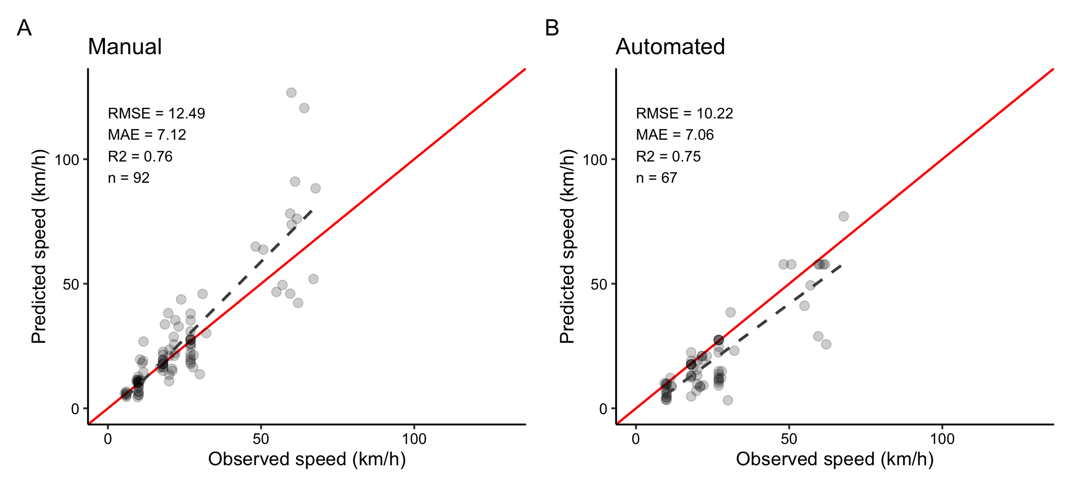

Figure 12: 1-to-1 plots of predicted vs observed boat speed estimates for **(A)** manual and **(B)** automated estimation methods. Dashed grey lines are linear regression trend lines; red lines indicate perfect agreement between predictions and observations.

The manual and automated 1-to-1 plots in Figure 12 are surprisingly similar. The manual method tended to overestimate speed, while the automated method underestimated. It appears that the manual plot is really thrown off by two high estimates. The automated method only matched 67 of the 92 boat passes though, and the logic of the matching loop likely prevented very high and very low estimates.

It’s appears that prediction error increases at higher speeds. We also notice that there are few trial runs between 30 and 50 km/h. Hard to validate if you don’t have a reference in that speed range.

Direction of Travel

Perhaps the navigation direction (upstream vs downstream) has an impact on estimation accuracy? Let’s check this for the automated results.

matched |> mutate(
  dir_label = recode(obs_dir,
                     "down" = "Downstream",
                     "up" = "Upstream")) |> 
  ggplot(aes(x = dir_label,
             y = speed_diff,
             fill = dir_label)) +
  geom_violin(show.legend = FALSE,
              alpha = 0.1) +
  geom_boxplot(show.legend = FALSE,
               alpha = 0.3,
               outliers = FALSE) +
  geom_jitter(aes(shape = dir_label),
              fill = NA,
              width = 0.08,
              alpha = 0.9,
              size = 2,
              show.legend = FALSE) +
  scale_shape_manual(values = c("Downstream" = 25, "Upstream" = 24)) +
  labs(title = "Prediction Error by Direction of Travel - Automated",
       x = NULL,
       y = "Prediction error (km/h)") +
  theme_bw(base_size = 14) +
   theme(
    axis.text.x = element_text(size = 14),
    axis.title.y = element_text(size = 14)
  )

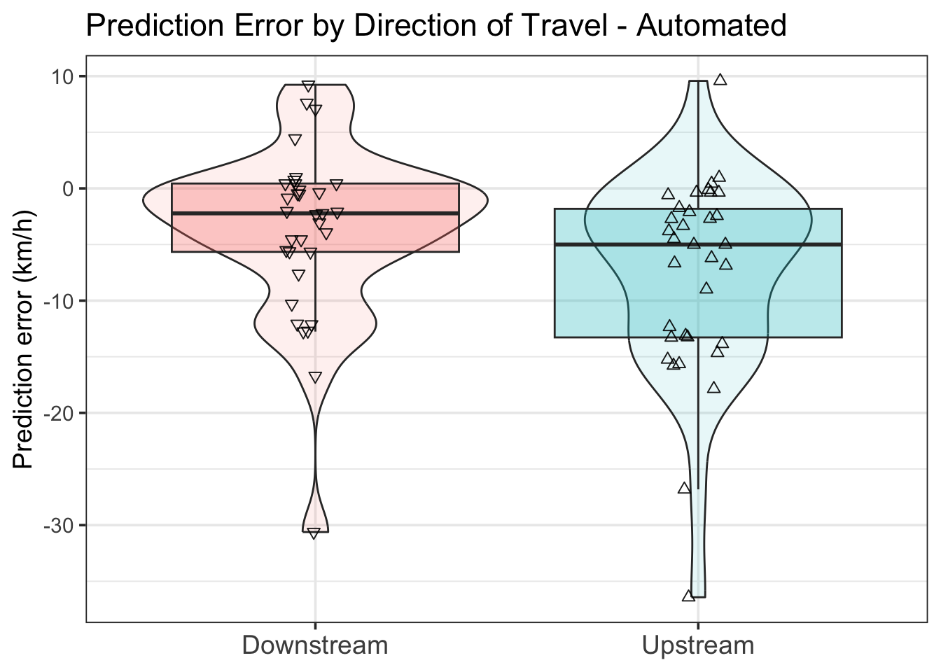
Figure 13: Boxplots and violin plots of boat speed prediction error based on direction of travel for n = 67 automated predictions. Thick black lines are median prediction error. Data points are shown as triangles with horizontal jittering to improve visualization.

We see from Figure 13 that median prediction error is lower for boats moving downstream compared to upstream, and again that speed underestimation is most common. Perhaps the bathymetry around the mics introduces a bias in directional sound propagation?

Prediction Error by Trial Day

Finally, let’s consider each day separately. Most importantly, this will indicate if boat type influences speed estimation.

counts <- matched |> 
  count(date) |> 
  mutate(date = factor(date))

matched |>
  mutate(date = factor(date)) |> 
  ggplot(aes(x = date,
             y = speed_diff,
             fill = date)) +
  geom_violin(show.legend = FALSE,
              alpha = 0.1) +
  geom_boxplot(show.legend = FALSE,
               alpha = 0.2,
               outliers = FALSE) +
  geom_jitter(fill = NA,
              width = 0.08,
              alpha = 0.5,
              size = 2,
              show.legend = FALSE) +
  geom_text(data = counts, aes(x = date, y = 17, label = paste0("n = ", n)),
            inherit.aes = FALSE, size = 4) +
  annotate("text", x = 1, y = 13, label = "Alumnium 14 ft") +
  annotate("text", x = 2, y = 13, label = "Wake surf 23 ft") +
  annotate("text", x = 3, y = 13, label = "Cruiser 28 ft") +
  labs(title = "Boat Speed Prediction Error by Day - Automated",
       x = "Date",
       y = "Prediction error (km/h)") +
  theme_bw(base_size = 14)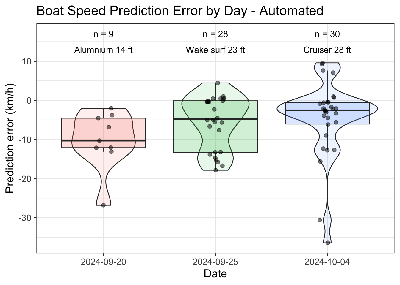

Figure 14: Boxplots and violin plots of boat speed prediction error based on day of sampling and boat type.

It appears that prediction accuracy improved as the trials went on. This may be because there sample size was larger for each subsequent day, or maybe we were getting better at our instrument deployments and observations. It may be influenced by the boat type being used: Sept 20 was a small vessel with a modest engine, while the other two boats had very powerful - and loud - engines.

Conclusion

This EDA sought to test if underwater acoustic recordings can be used for accurate estimation of boat speed and if it can be done reliably without user oversight. The broad takeaway from this analysis is that, yes, I was able to produce reasonable speed estimates; however, the method is not currently accurate enough to be put into practice. But it shows promise. Honestly, I’m a little shocked that the automated method had lower error metrics (RMSE = 10.22 km/h, MAE = 7.06 km/h) than the manual approach (RMSE = 12.49 km/h, MAE = 7.12 km/h). But take these results with a grain of salt, as the manual approach had no temporal limits on the matching. If the two obvious outliers are removed from the manual results, it shows better than the automated approach. And, the manual approach had an estimate for every boat pass, while the automated method only generated estimates for 73% of passes.

Another key consideration is that these trials were purposely designed to limit interference from other boats – basically ideal testing conditions. Both methods would likely yield considerably poorer results during periods of high traffic.

As currently developed, this automated boat speed estimator can provide moderate accuracy of boat speed and would be appropriate for categories of speed (e.g., between 10 and 30 km/h). However, it is not able generate sufficiently accurate speeds estimates suitable as input for numeric models of boat wake generation.

And so:

RQ1: Yes, we can definitely estimate boat speed from underwater acoustic recordings.

RQ2: Yes, the process can be fully-automated in R and yield similar accuracy to a manual approach.

RQ3: No, as currently developed, the automated method is not yet ready for upscaling and adoption for 2025. But, I’ve got another 6 weeks to refine it…

Artificial Intelligence Usage Statement

Some of the custom functions developed for my research are at a level of complexity beyond my programming skills. I have troubleshooted many of these functions with the assistance of OpenAI’s ChatGPT (OpenAI, 2024). I have found this process to be rewarding, but also demanding, and I have full records of these coding sessions. These custom functions have allowed me to produce the results that I then personally prepared for this report.

References

Audacity Team. (2025). Audacity: Free audio editor and recorder. https://www.audacityteam.org/

Forlini, C., Qayyum, R., Malej, M., Lam, M.-A. Y.-H., Shi, F., Angelini, C., & Sheremet, A. (2021). On the problem of modeling the boat wake climate: The Florida Intracoastal Waterway. Journal of Geophysical Research: Oceans, 126(2), e2020JC016676. https://doi.org/10.1029/2020JC016676

Gabel, F., Lorenz, S., & Stoll, S. (2017). Effects of ship-induced waves on aquatic ecosystems. Science of The Total Environment, 601-602, 926–939. https://doi.org/10.1016/j.scitotenv.2017.05.206

Hill, A. P., Prince, P., Piña Covarrubias, E., Doncaster, C. P., Snaddon, J. L., & Rogers, A. (2018). AudioMoth: Evaluation of a smart open acoustic device for monitoring biodiversity and the environment. Methods in Ecology and Evolution, 9(5), 1199–1211. https://doi.org/10.1111/2041-210X.12955

Lamont, T. A. C., Chapuis, L., Williams, B., Dines, S., Gridley, T., Frainer, G., Fearey, J., Maulana, P. B., Prasetya, M. E., Jompa, J., Smith, D. J., & Simpson, S. D. (2022). HydroMoth: Testing a prototype low-cost acoustic recorder for aquatic environments. Remote Sensing in Ecology and Conservation, 8(3), 362–378. https://doi.org/10.1002/rse2.249

OpenAI. (2024). ChatGPT (april 2024 version). https://chat.openai.com

R Core Team. (2025). R: A language and environment for statistical computing. R Foundation for Statistical Computing. https://www.R-project.org/

Schafft, M., Wegner, B., Meyer, N., Wolter, C., & Arlinghaus, R. (2021). Ecological impacts of water-based recreational activities on freshwater ecosystems: a global meta-analysis. Proceedings of the Royal Society B: Biological Sciences, 288(1959), 20211623. https://doi.org/10.1098/rspb.2021.1623

Shannon, C. E. (1949). Communication in the presence of noise. Proceedings of the IRE, 37(1), 10–21. https://doi.org/10.1109/JRPROC.1949.232969

Sueur, J. (2018). Sound analysis and synthesis with r. Springer International Publishing. https://doi.org/10.1007/978-3-319-77647-7

Sueur, J., Aubin, T., & Simonis, C. (2008). Seewave: A free modular tool for sound analysis and synthesis. Bioacoustics, 18(2), 213–226. https://doi.org/10.1080/09524622.2008.9753600