Effect of Pavement on the Number of Wildlife Roadkills

Author

Marina de Souza

Data Collection Context

Brazilian legislation, through the environmental licensing process, requires a series of studies to be conducted for different types of infrastructure projects, such as highways. In this context, studies are often focused on understanding the spatial patterns of wildlife-vehicle collision hotspots, with the aim of guiding the implementation of mitigation measures.

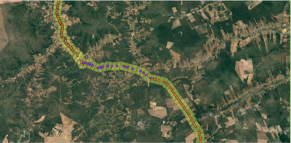
Within this framework, we recorded wildlife impacted by vehicle collisions along the BR-135 highway, located in western Bahia and northern Minas Gerais, in a transitional area between the Cerrado and Caatinga biomes.

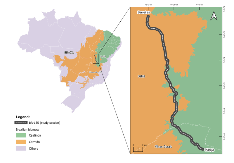
Over a period of five years, we conducted monthly surveys using a vehicle traveling at speeds between 40–60 km/h, covering nearly 370 km of roadway. This stretch includes both paved and unpaved segments. As a result, the dataset includes records of amphibians, birds, reptiles, and mammals affected by vehicle collisions.

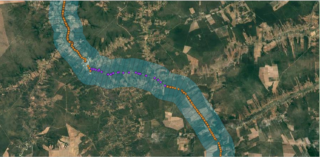
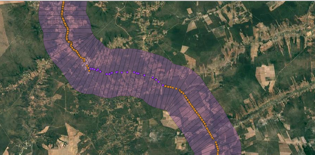
To account for how landscape composition might influence roadkill events, we extracted land use and land cover data from the MapBiomas platform (https://brasil.mapbiomas.org/) at three spatial scales from the road axis: 1 km, 3 km, and 5 km. Additionally, traffic volume data were incorporated—field-collected data were available for one segment, while for the remaining segments, traffic volume estimates were obtained through models provided by the Brazilian National Department of Transport Infrastructure (DNIT).

Using the spatialized information, we clipped the polygons derived at the 1 km scale so that each polygon had an area of 2 km². For the 3 km scale, each polygon covered an area of 6 km², and for the 5 km scale, each polygon covered 10 km².

Goals

The objective of this document is to prepare the dataset and subsequently investigate the effect of road pavement on the number of wildlife roadkills.

1) Is there an effect of pavement on the number of wildlife roadkills?

Hypothesis: Considering that pavement allows vehicles to travel at higher speeds and is also associated with increased traffic volume, we expect a higher number of roadkills in paved areas.

2) Does the influence of pavement on the number of roadkill records differ among taxonomic groups?

Hypothesis: Considering that pavement affects vehicle speed, we expect a more pronounced increase in roadkills of more mobile groups, such as birds and mammals, compared to amphibians and reptiles.

3) Do dry and rainy seasons in this region of Brazil influence the number of recorded wildlife roadkills?

Hypothesis: We predict higher roadkill rates during the rainy season due to increased wildlife activity driven by warmer temperatures

4) Does the variation in the spatial scale used to assess landscape components (1 km, 3 km, and 5 km) reflect differences in their relationship with the number of roadkills?

Hypothesis: At larger spatial scales, considering that the total amount of habitat tends to increase, we expect landscape components to have a stronger influence on the number of roadkills. This influence is expected to occur in both the overall roadkill analyses and those conducted separately for each taxonomic group.

Description of the Data Structure

This dataset contains information on roadkill occurrences across different road segments, categorized by taxonomic group, seasonality, and various environmental and infrastructural variables. The dataset includes the following columns:

Variable	Description
polygon	Identifier for the road and landscape segment.
taxa	Taxonomic group of the affected species (e.g., mammals, reptiles, amphibians, birds).
season	Season in which the observation was recorded (dry or rainy).
roadkill_count	Number of roadkill occurrences recorded in the segment/taxa/season.
road_length	Length of the road segment (in kilometers).
relative_rate	A measure of roadkill occurrences relative to the road length.
cult_land	Proportion of cultivated land within the segment’s surrounding area.
water	Proportion of water bodies within the segment’s surrounding area.
shrubby	Proportion of shrubby vegetation within the segment’s surrounding area.
pasture	Proportion of pastureland within the segment’s surrounding area.
urban_area	Proportion of urbanized area within the segment’s surrounding area.
forest	Proportion of forested land within the segment’s surrounding area.
savanna	Proportion of savanna within the segment’s surrounding area.
pavement	Proportion of paved road surface.
traffic	A measure of traffic intensity in the road segment.

Packages

library(openxlsx)
library(dplyr)
library(vegan)
library(ggplot2)
library(tidyr)
library(lattice)
library(purrr)
library(rlang)
library(corrplot)
library(MASS)
library(DHARMa)
library(gridExtra)
library(grid)
library(performance)
library(piecewiseSEM)
library(emmeans) 
library(car)
library(lme4)
library(glmmTMB)
library(AICcmodavg)
library(MuMIn)
library(bbmle)
library(grid)
library(tree)
library(writexl)
library(sjPlot)
library(patchwork)
library(ggeffects)
library(visreg)
library(broom.mixed)
library(cowplot)

Datasets

d1km_raw <- read.xlsx("data_1km.xlsx")
d3km_raw <- read.xlsx("data_3km.xlsx")
d5km_raw <- read.xlsx("data_5km.xlsx")

Pavement as a binary variable

Since the pavement variable is in proportion but is mostly a binary variable, we will exclude polygons with intermediate values (where the road segment is partially paved and partially unpaved). I want to keep only the rows where the values are exactly 0 or 1, and exclude all rows with intermediate values, i.e., values greater than 0 and less than 1.

d1km_raw <- d1km_raw %>% filter(pavement %in% c(0, 1))
d3km_raw <- d3km_raw %>% filter(pavement %in% c(0, 1))
d5km_raw <- d5km_raw %>% filter(pavement %in% c(0, 1))

checking the values

all(d1km_raw$pavement %in% c(0, 1))

[1] TRUE

all(d3km_raw$pavement %in% c(0, 1))

[1] TRUE

all(d5km_raw$pavement %in% c(0, 1))

[1] TRUE

Data detailed by taxon and season

I’ll create a list containing the three datasets to simplify the required data manipulation

datasets_raw <- list("1km" = d1km_raw, "3km" = d3km_raw, "5km" = d5km_raw)

Now that all the data has been prepared, we can combine the 1 km, 3 km, and 5 km datasets into a single dataframe, while keeping a column to identify the scale

combined_raw <- bind_rows(
  d1km_raw %>% mutate(scale = "1km"),
  d3km_raw %>% mutate(scale = "3km"),
  d5km_raw %>% mutate(scale = "5km")
)

To ensure that categorical and numerical variables are properly recognized by R

combined_raw$polygon <- as.factor(combined_raw$polygon)
combined_raw$taxa <- factor(combined_raw$taxa, levels=c("amp","rep", "bird", "mam"))
combined_raw$season <- factor(combined_raw$season, levels=c("dry","rainy"))
combined_raw$pavement <- factor(combined_raw$pavement, levels=c("0","1"))
combined_raw$traffic <- factor(combined_raw$traffic, levels=c("low", "medium","high"), ordered = TRUE)
str(combined_raw)

'data.frame':   8808 obs. of  16 variables:
 $ polygon       : Factor w/ 376 levels "1","2","3","4",..: 1 1 1 1 1 1 1 1 2 2 ...
 $ taxa          : Factor w/ 4 levels "amp","rep","bird",..: 4 4 2 2 1 1 3 3 4 4 ...
 $ season        : Factor w/ 2 levels "dry","rainy": 1 2 1 2 1 2 1 2 1 2 ...
 $ roadkill_count: num  0 0 0 0 0 0 0 0 1 0 ...
 $ road_length   : num  1.02 1.02 1.02 1.02 1.02 ...
 $ relative_rate : num  0 0 0 0 0 ...
 $ cult_land     : num  0.23 0.23 0.23 0.23 0.23 ...
 $ water         : num  0.0654 0.0654 0.0654 0.0654 0.0654 ...
 $ shrubby       : num  0 0 0 0 0 0 0 0 0 0 ...
 $ pasture       : num  0.0139 0.0139 0.0139 0.0139 0.0139 ...
 $ urban_area    : num  1.41 1.41 1.41 1.41 1.41 ...
 $ forest        : num  0.0874 0.0874 0.0874 0.0874 0.0874 ...
 $ savanna       : num  0.18 0.18 0.18 0.18 0.18 ...
 $ pavement      : Factor w/ 2 levels "0","1": 2 2 2 2 2 2 2 2 2 2 ...
 $ traffic       : Ord.factor w/ 3 levels "low"<"medium"<..: 3 3 3 3 3 3 3 3 3 3 ...
 $ scale         : chr  "1km" "1km" "1km" "1km" ...

General data without distinguishing between taxa or seasons

Combine the records of roadkill regardless of rate and season; therefore, we will group by polygon. The roadkill count should be summarized, and for the other columns, we will keep only the first row of each polygon, as as the others are identical copies of the first.

summarize_dataset <- function(data) {
  data %>%
    group_by(polygon) %>%
    summarise(
      total_roadkill_count = sum(roadkill_count),
      road_length = first(road_length),
      cult_land = first(cult_land),
      water = first(water),
      shrubby = first(shrubby),
      pasture = first(pasture),
      urban_area = first(urban_area), 
      forest = first(forest),
      savanna = first(savanna),
      pavement = first(pavement), 
      traffic = first(traffic),
      .groups = "drop"
    )
}

sum_datasets <- lapply(datasets_raw, summarize_dataset)

d1km_raw_sum <- sum_datasets[[1]]
d3km_raw_sum <- sum_datasets[[2]]
d5km_raw_sum <- sum_datasets[[3]]

Data Exploration

General exploration - dataset with taxa and season

Now that the data has been reorganized, let’s perform some exploratory analyses and transformations.

Let’s create histograms of the variables to get an idea of their distribution.

numeric_vars <- c("roadkill_count", "road_length", "relative_rate", 
                  "cult_land", "water", "shrubby", "pasture", 
                  "urban_area", "forest", "savanna")

long_numeric <- combined_raw |>
  tidyr::pivot_longer(cols = all_of(numeric_vars),
                      names_to = "variable", values_to = "value") |>
  dplyr::select(scale, variable, value)

plot_histograms <- function(scale_level) {
  color_map <- c("1km" = "#FFD700", "3km" = "#1f77b4", "5km" = "#9B59B6")
  
  long_numeric %>%
    filter(scale == scale_level) %>%
    ggplot(aes(x = value)) +
    geom_bar(data = ~ filter(., variable == "traffic"),
             fill = color_map[[scale_level]], color = "white") +
    geom_histogram(data = ~ filter(., variable != "traffic"),
                   bins = 30, fill = color_map[[scale_level]], color = "white") +
    facet_wrap(~ variable, scales = "free", ncol = 4) +
    labs(title = paste("Histograms -", scale_level),
         x = NULL, y = "frequency") +
    theme_minimal()
}

plot_1km <- plot_histograms("1km")
plot_3km <- plot_histograms("3km")
plot_5km <- plot_histograms("5km")

plot_1km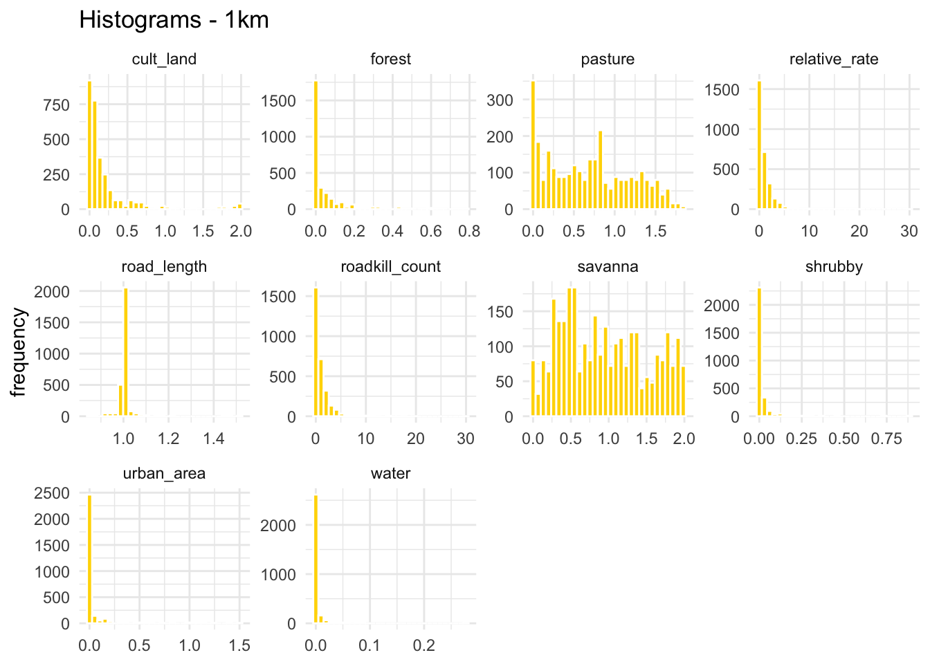

plot_3km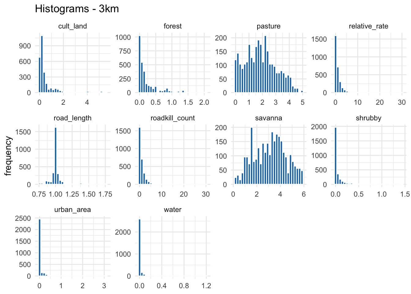

plot_5km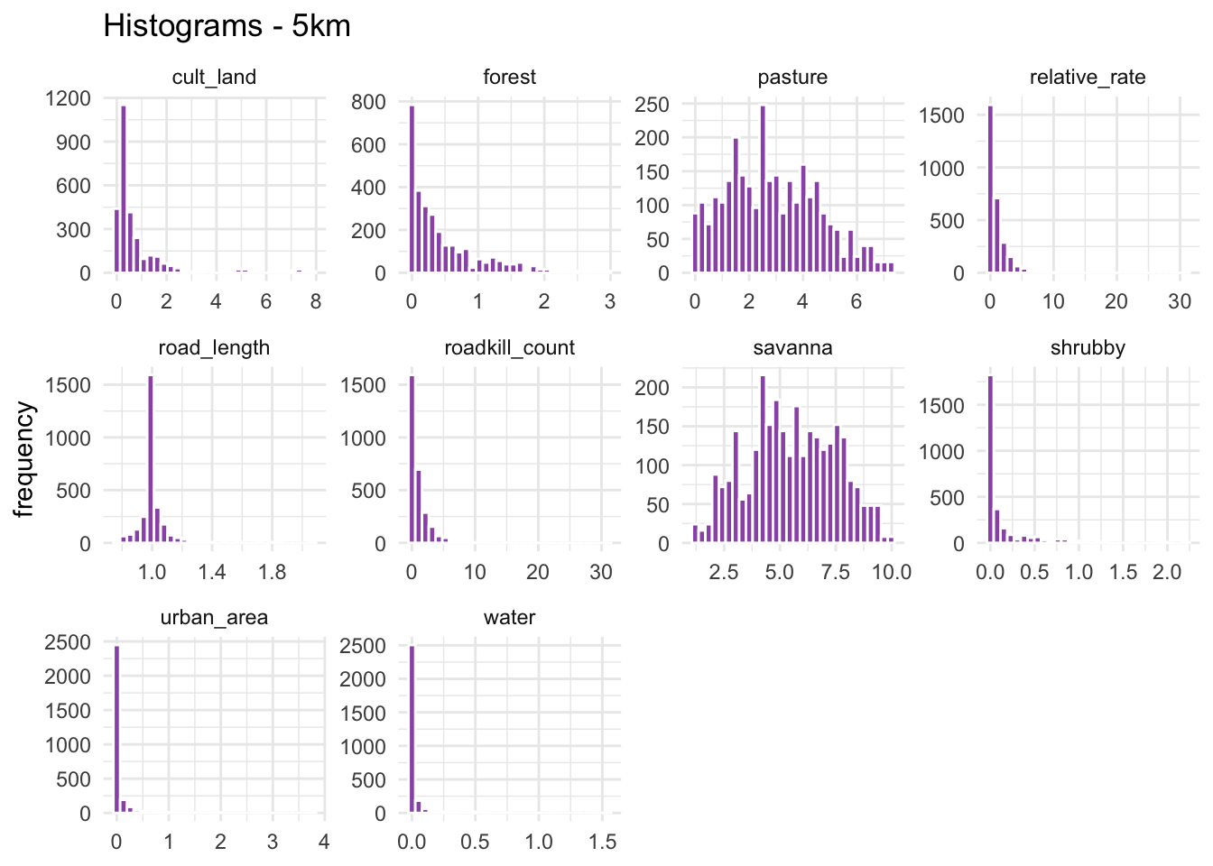

Since the traffic and pavement variables are the same across all subsets, the histograms should look identical for each scale. Let’s generate the histograms to confirm that this information is indeed consistent across the three datasets.

ggplot(combined_raw, aes(x = traffic, fill = interaction(traffic, scale))) +
  geom_bar() +
  facet_wrap(~ scale) +
  theme_minimal() +
  labs(
    title = "Traffic category frequency by scale",
    x = "Traffic category",
    y = "Frequency"
  ) +
  scale_fill_manual(values = c(
   
    "low.1km" = "#FFF8B0",    
    "medium.1km" = "#FFD700", 
    "high.1km" = "#E6BE00",   

   
    "low.3km" = "#AED6F1",    
    "medium.3km" = "#1f77b4", 
    "high.3km" = "#154360",   

    
    "low.5km" = "#E8DAEF",    
    "medium.5km" = "#9B59B6", 
    "high.5km" = "#6C3483"    
  )) + 
  theme(legend.position="none")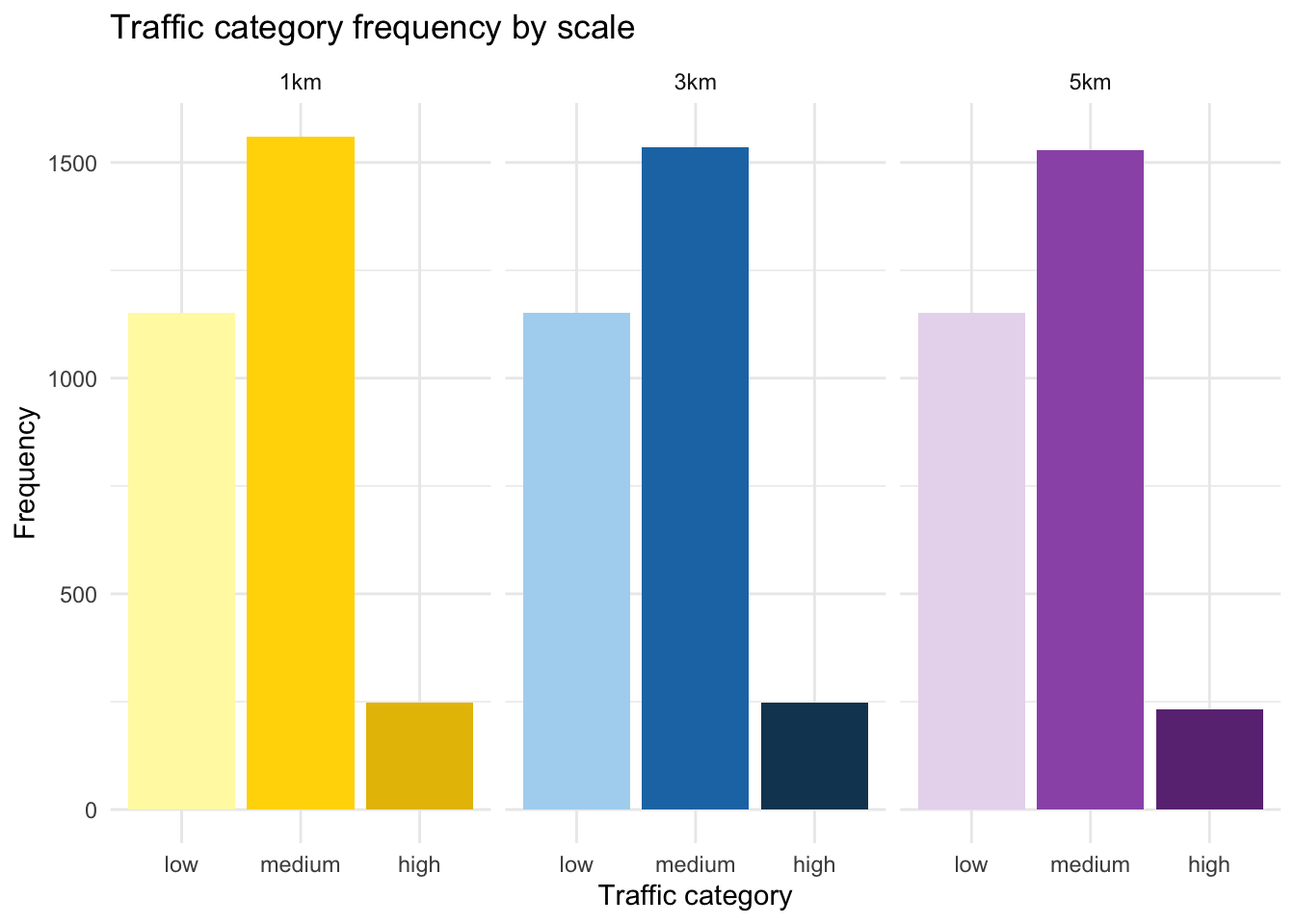

ggplot(combined_raw, aes(x = pavement, fill = interaction(pavement, scale))) +
  geom_bar() +
  facet_wrap(~ scale) +
  theme_minimal() +
  labs(
    title = "Pavement category frequency by scale",
    x = "Pavement category",
    y = "Frequency"
  ) +
  scale_fill_manual(values = c(
    "0.1km" = "#FFD700",
    "1.1km" = "#E6BE00",
    "0.3km" = "#1f77b4",
    "1.3km" = "#154360",
    "0.5km" = "#9B59B6",
    "1.5km" = "#6C3483"
  )) +
  theme(legend.position = "none")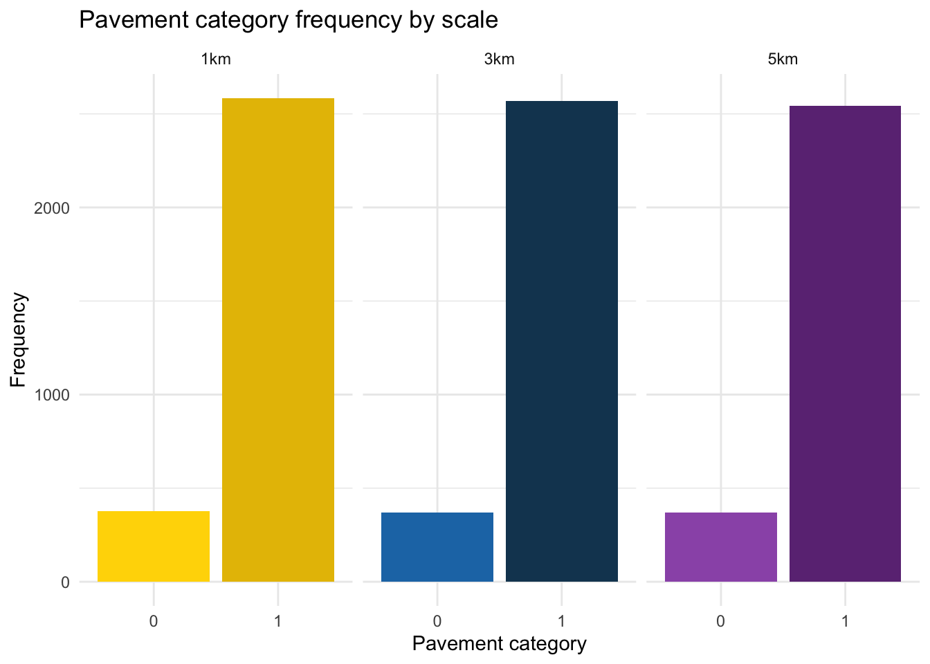

Is there collinearity among the covariates?

Collinearity was assessed to avoid redundancy among covariates, which can affect model stability and interpretation.

check_collinearity <- function(data, scale_label) {
  landscape_vars <- data %>%
    dplyr::select(cult_land, water, shrubby, pasture, urban_area, forest, savanna)
  
  cor_matrix <- cor(landscape_vars, use = "complete.obs")
  
  colors_1km <- c("low.1km" = "#FFF8B0", "medium.1km" = "#FFD700", "high.1km" = "#E6BE00")
  colors_3km <- c("low.3km" = "#AED6F1", "medium.3km" = "#1f77b4", "high.3km" = "#154360")
  colors_5km <- c("low.5km" = "#E8DAEF", "medium.5km" = "#9B59B6", "high.5km" = "#6C3483")
  
    if (scale_label == "1 km") {
    corrplot(cor_matrix,
             method = "color",
             type = "upper",
             tl.col = "black",
             tl.srt = 45,
             addCoef.col = "black",
             col = colors_1km,
             title = paste("Collinearity -", scale_label),
             mar = c(0,0,2,0))
  } else if (scale_label == "3 km") {
    corrplot(cor_matrix,
             method = "color",
             type = "upper",
             tl.col = "black",
             tl.srt = 45,
             addCoef.col = "black",
             col = colors_3km,
             title = paste("Collinearity -", scale_label),
             mar = c(0,0,2,0))
  } else if (scale_label == "5 km") {
    corrplot(cor_matrix,
             method = "color",
             type = "upper",
             tl.col = "black",
             tl.srt = 45,
             addCoef.col = "black",
             col = colors_5km,
             title = paste("Collinearity -", scale_label),
             mar = c(0,0,2,0))
  }
}

# Aplicar para cada escala
check_collinearity(d1km_raw, "1 km")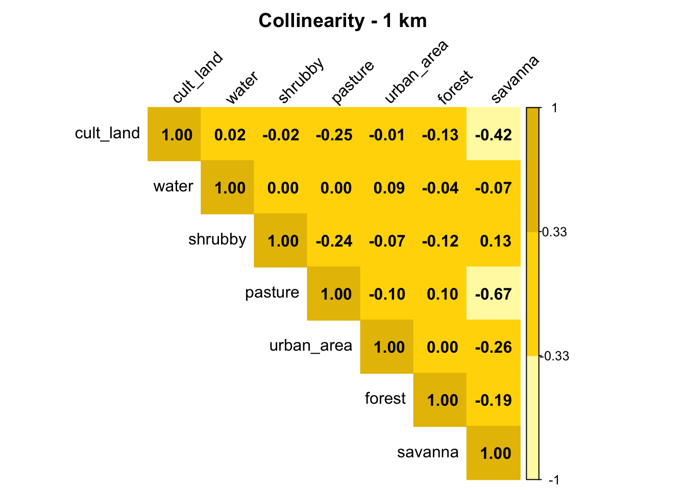

check_collinearity(d3km_raw, "3 km")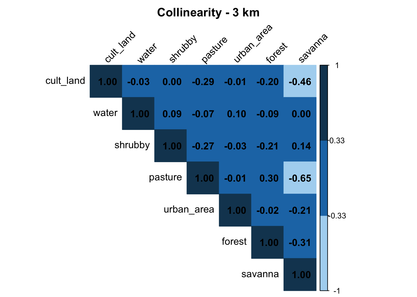

check_collinearity(d5km_raw, "5 km")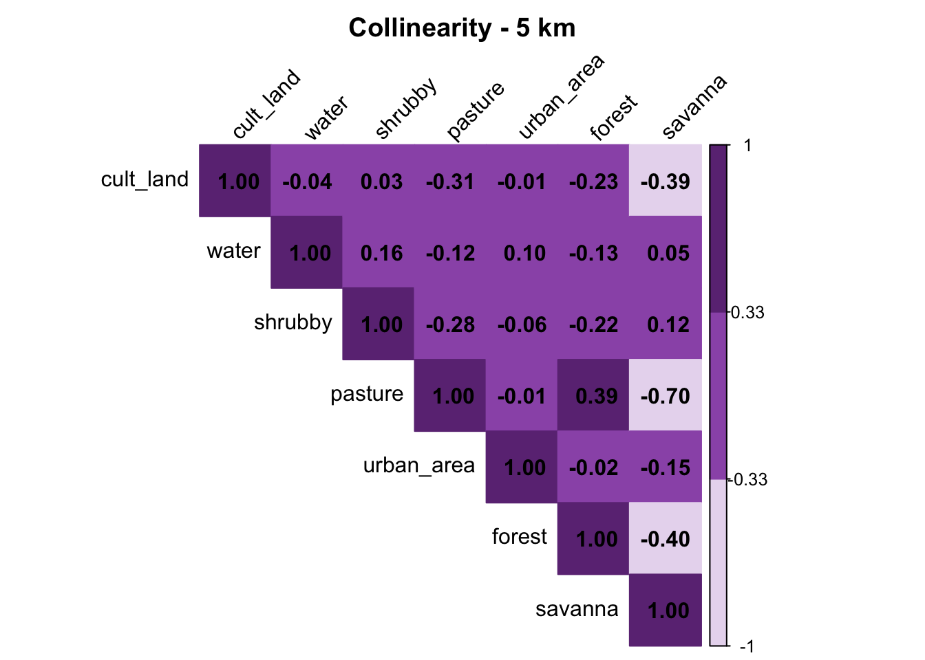

Pasture and savanna are highly correlated, so we don’t need to include both of these variables in our model.

Transformations

Due to the heterogeneity in the scales at which the exploratory variables were measured, and aiming to reduce the effect of outliers, the values will be transformed by applying the logarithmic transformation for variables in m² and square root for linear variables. To make variables comparable and ensure they contribute equally to the analysis, all transformed variables were then standardized using z-score normalization (mean = 0, standard deviation = 1).

The datasets, disaggregated by taxon and season, that have been transformed and standardized will be referred to as d1km, d3km, and d5km. The datasets containing the total number of roadkills (without separating by taxon or season) will be named 1km_sum, 3km_sum, and 5km_sum.

Log

vars_to_log <- c("cult_land", "water", "shrubby", "pasture", 
                 "urban_area", "forest", "savanna")

datasets_t <- lapply(datasets_raw, function(data) {
  data %>%
    mutate(across(all_of(vars_to_log), ~ log(.x + 1)))
})

d1km <- datasets_t[[1]]
d3km <- datasets_t[[2]]
d5km <- datasets_t[[3]]


datasets_sum_t <- lapply(sum_datasets, function(data) {
  data %>%
    mutate(across(all_of(vars_to_log), ~ log(.x + 1)))
})

d1km_sum <- datasets_sum_t[[1]]
d3km_sum <- datasets_sum_t[[2]]
d5km_sum <- datasets_sum_t[[3]]

Square root

vars_to_sqrt <- c("road_length") 

datasets_t <- map(datasets_t, ~ .x %>%
                  mutate(across(all_of(vars_to_sqrt), ~ sqrt(.x))))

d1km <- datasets_t[[1]]
d3km <- datasets_t[[2]]
d5km <- datasets_t[[3]]


datasets_sum_t <- map(datasets_sum_t, ~ .x %>%
                  mutate(across(all_of(vars_to_sqrt), ~ sqrt(.x))))

d1km_sum <- datasets_sum_t[[1]]
d3km_sum <- datasets_sum_t[[2]]
d5km_sum <- datasets_sum_t[[3]]

z-score standardization

vars_to_standardize <- c("cult_land", "water", "shrubby", "pasture", 
                         "urban_area", "forest", "savanna", "road_length")

datasets_t <- lapply(datasets_t, function(data) {
  data %>%
    mutate(across(all_of(vars_to_standardize), ~ decostand(.x, method = "standardize")))
})

d1km <- datasets_t[[1]]
d3km <- datasets_t[[2]]
d5km <- datasets_t[[3]]

datasets_sum_t <- lapply(datasets_sum_t, function(data) {
  data %>%
    mutate(across(all_of(vars_to_standardize), ~ decostand(.x, method = "standardize")))
})

d1km_sum <- datasets_sum_t[[1]]
d3km_sum <- datasets_sum_t[[2]]
d5km_sum <- datasets_sum_t[[3]]

Statistical Analyses - GLM e GLMM

It is worth noting that the selected analyses presented here underwent a prior selection process to determine the distribution family that best fit our data. The models used for analyses involving the total number of roadkills (i.e., without separation by taxonomic group) are referred to as total_Xkm_mx. For example, the global model using the total number of roadkill records at the 1 km scale is named total_1km_m0. In contrast, the model in which records are separated by taxon is called taxa_Xkm_mX. If model selection is applied within each analysis (e.g., variable removal), the final number in the model name will reflect the changes made in relation to the global model m0.

Total number of roadkill

We want to assess how pavement affects the number of recorded roadkill incidents, regardless of the season or taxonomic group.

VARIABLES

Response variable: Roadkill number

Predictor variable: Pavement as binary

Exploratory variables: Road length; Cultivated land; Water; Shrubby; Pasture*; Urban area; Forest; Savanna and Traffic.

*It were excluded of model due to correlation with Savanna

Since we performed many transformations after initially specifying the nature of the data, it’s better to double-check that everything is still correctly defined

format_data_GLM <- function(df) {
  df$polygon <- as.factor(df$polygon)
  df$pavement <- factor(df$pavement, levels = c("0", "1"))
  df$traffic <- factor(df$traffic, levels = c("low", "medium", "high"), ordered = TRUE)
  df$water <- as.numeric(df$water)
  df$road_length <- as.numeric(df$road_length)
  df$shrubby <- as.numeric(df$shrubby)
  df$urban_area <- as.numeric(df$urban_area)
  df$cult_land <- as.numeric(df$cult_land)
  df$savanna <- as.numeric(df$savanna)
  df$forest <- as.numeric(df$forest)
  df$p <- as.numeric(df$savanna)
  return(df)
}

# Aplicar aos datasets
d1km_sum <- format_data_GLM(d1km_sum)
d3km_sum <- format_data_GLM(d3km_sum)
d5km_sum <- format_data_GLM(d5km_sum)

GLM - Negative binomial

We started the analysis by considering traffic as a random effect in a GLMM. At first, we tried a Poisson model, but it showed signs of overdispersion. Still keeping traffic as a random effect, we then tried a negative binomial model, which handles overdispersion better. However, it was not possible to fit the model properly. Therefore, we present here a negative binomial GLM, treating traffic as a fixed effect.

1km

Global model

total_1km_m0 <- glm.nb (total_roadkill_count ~  traffic + pavement + road_length + cult_land + forest+ urban_area + water + shrubby + savanna, 
              data = d1km_sum)

Overdispersion

(chat <- deviance(total_1km_m0) / df.residual(total_1km_m0))

[1] 1.100957

Model selection using drop1

We used the drop1 function in R to compare nested models and identify the most influential predictors. This function tests the effect of removing each term from the full model, one at a time, using likelihood ratio tests. Variables with higher p-values contribute less to the model, so we progressively removed the least significant terms, keeping those with the lowest p-values to improve model parsimony. The same procedure will be applied to the other spacial scales.

Global model

drop1(total_1km_m0, test="Chi")

Single term deletions

Model:
total_roadkill_count ~ traffic + pavement + road_length + cult_land + 
    forest + urban_area + water + shrubby + savanna
            Df Deviance    AIC     LRT  Pr(>Chi)    
<none>           395.24 2052.9                      
traffic      2   568.11 2221.8 172.863 < 2.2e-16 ***
pavement     1   500.46 2156.2 105.219 < 2.2e-16 ***
road_length  1   396.30 2052.0   1.060   0.30313    
cult_land    1   398.54 2054.2   3.298   0.06938 .  
forest       1   395.26 2050.9   0.018   0.89247    
urban_area   1   432.89 2088.6  37.647  8.48e-10 ***
water        1   396.27 2052.0   1.025   0.31142    
shrubby      1   397.23 2052.9   1.986   0.15878    
savanna      1   411.83 2067.5  16.590  4.64e-05 ***
---
Signif. codes:  0 '***' 0.001 '**' 0.01 '*' 0.05 '.' 0.1 ' ' 1

without forest

total_1km_m1 <- glm.nb (total_roadkill_count ~ traffic + pavement + urban_area + water +
                cult_land + shrubby + savanna + road_length,data = d1km_sum)
drop1(total_1km_m1, test="Chi")

Single term deletions

Model:
total_roadkill_count ~ traffic + pavement + urban_area + water + 
    cult_land + shrubby + savanna + road_length
            Df Deviance    AIC     LRT  Pr(>Chi)    
<none>           395.26 2050.9                      
traffic      2   568.20 2219.9 172.946 < 2.2e-16 ***
pavement     1   500.46 2154.2 105.206 < 2.2e-16 ***
urban_area   1   433.18 2086.9  37.925 7.351e-10 ***
water        1   396.29 2050.0   1.030   0.31010    
cult_land    1   398.55 2052.2   3.299   0.06932 .  
shrubby      1   397.22 2050.9   1.968   0.16071    
savanna      1   412.21 2065.9  16.957 3.824e-05 ***
road_length  1   396.31 2050.0   1.055   0.30426    
---
Signif. codes:  0 '***' 0.001 '**' 0.01 '*' 0.05 '.' 0.1 ' ' 1

without water

total_1km_m2 <- glm.nb (total_roadkill_count ~ traffic + pavement + urban_area +
                cult_land + shrubby + savanna + road_length,data = d1km_sum)
drop1(total_1km_m2, test="Chi")

Single term deletions

Model:
total_roadkill_count ~ traffic + pavement + urban_area + cult_land + 
    shrubby + savanna + road_length
            Df Deviance    AIC     LRT  Pr(>Chi)    
<none>           395.04 2050.0                      
traffic      2   591.37 2242.3 196.327 < 2.2e-16 ***
pavement     1   502.17 2155.1 107.122 < 2.2e-16 ***
urban_area   1   433.51 2086.4  38.465 5.576e-10 ***
cult_land    1   398.72 2051.7   3.672   0.05532 .  
shrubby      1   396.85 2049.8   1.810   0.17855    
savanna      1   412.77 2065.7  17.730 2.546e-05 ***
road_length  1   396.05 2049.0   1.009   0.31525    
---
Signif. codes:  0 '***' 0.001 '**' 0.01 '*' 0.05 '.' 0.1 ' ' 1

without road length

total_1km_m3 <- glm.nb (total_roadkill_count ~ traffic + pavement + urban_area +
                cult_land + shrubby + savanna, data = d1km_sum)
drop1(total_1km_m3, test="Chi")

Single term deletions

Model:
total_roadkill_count ~ traffic + pavement + urban_area + cult_land + 
    shrubby + savanna
           Df Deviance    AIC     LRT  Pr(>Chi)    
<none>          395.71 2049.0                      
traffic     2   594.68 2243.9 198.967 < 2.2e-16 ***
pavement    1   501.84 2153.1 106.128 < 2.2e-16 ***
urban_area  1   433.74 2085.0  38.030 6.966e-10 ***
cult_land   1   399.55 2050.8   3.836   0.05015 .  
shrubby     1   397.20 2048.5   1.490   0.22229    
savanna     1   413.97 2065.2  18.261 1.926e-05 ***
---
Signif. codes:  0 '***' 0.001 '**' 0.01 '*' 0.05 '.' 0.1 ' ' 1

without shrubby

total_1km_m4 <- glm.nb (total_roadkill_count ~ traffic + pavement + urban_area +
                cult_land + savanna, data = d1km_sum)

drop1(total_1km_m4, test="Chi")

Single term deletions

Model:
total_roadkill_count ~ traffic + pavement + urban_area + cult_land + 
    savanna
           Df Deviance    AIC     LRT  Pr(>Chi)    
<none>          394.16 2048.5                      
traffic     2   599.21 2249.5 205.049 < 2.2e-16 ***
pavement    1   507.56 2159.9 113.394 < 2.2e-16 ***
urban_area  1   432.05 2084.3  37.890 7.483e-10 ***
cult_land   1   398.45 2050.8   4.289   0.03835 *  
savanna     1   414.32 2066.6  20.154 7.147e-06 ***
---
Signif. codes:  0 '***' 0.001 '**' 0.01 '*' 0.05 '.' 0.1 ' ' 1

without cultivated land

total_1km_m5 <- glm.nb (total_roadkill_count ~ traffic + pavement + urban_area
                 + savanna, data = d1km_sum)
drop1(total_1km_m5, test="Chi")

Single term deletions

Model:
total_roadkill_count ~ traffic + pavement + urban_area + savanna
           Df Deviance    AIC     LRT  Pr(>Chi)    
<none>          393.57 2050.7                      
traffic     2   605.64 2258.8 212.077 < 2.2e-16 ***
pavement    1   502.10 2157.2 108.538 < 2.2e-16 ***
urban_area  1   427.41 2082.6  33.848 5.960e-09 ***
savanna     1   409.45 2064.6  15.885 6.732e-05 ***
---
Signif. codes:  0 '***' 0.001 '**' 0.01 '*' 0.05 '.' 0.1 ' ' 1

without savanna

total_1km_m6 <- glm.nb (total_roadkill_count ~ traffic + pavement + urban_area,
                        data = d1km_sum)
drop1(total_1km_m6, test="Chi")

Single term deletions

Model:
total_roadkill_count ~ traffic + pavement + urban_area
           Df Deviance    AIC     LRT  Pr(>Chi)    
<none>          393.36 2064.2                      
traffic     2   600.82 2267.7 207.462 < 2.2e-16 ***
pavement    1   500.09 2168.9 106.735 < 2.2e-16 ***
urban_area  1   418.01 2086.9  24.651 6.869e-07 ***
---
Signif. codes:  0 '***' 0.001 '**' 0.01 '*' 0.05 '.' 0.1 ' ' 1

without urban area

total_1km_m7 <- glm.nb (total_roadkill_count ~ traffic + pavement,
                        data = d1km_sum)
drop1(total_1km_m7, test="Chi")

Single term deletions

Model:
total_roadkill_count ~ traffic + pavement
         Df Deviance    AIC     LRT  Pr(>Chi)    
<none>        390.44 2085.8                      
traffic   2   566.42 2257.7 175.980 < 2.2e-16 ***
pavement  1   485.27 2178.6  94.827 < 2.2e-16 ***
---
Signif. codes:  0 '***' 0.001 '**' 0.01 '*' 0.05 '.' 0.1 ' ' 1

without traffic

total_1km_m8 <- glm.nb (total_roadkill_count ~ pavement, data = d1km_sum)
drop1(total_1km_m8, test="Chi")

Single term deletions

Model:
total_roadkill_count ~ pavement
         Df Deviance    AIC    LRT  Pr(>Chi)    
<none>        390.65 2221.2                     
pavement  1   488.03 2316.6 97.378 < 2.2e-16 ***
---
Signif. codes:  0 '***' 0.001 '**' 0.01 '*' 0.05 '.' 0.1 ' ' 1

3km

total_3km_m0 <- glm.nb (total_roadkill_count ~ traffic + pavement + savanna + urban_area +
                          water + forest + road_length + cult_land  + shrubby, 
              data = d3km_sum)

Overdispersion

(chat <- deviance(total_3km_m0) / df.residual(total_3km_m0))

[1] 1.106621

Model selection using drop1

drop1(total_3km_m0, test="Chi")

Single term deletions

Model:
total_roadkill_count ~ traffic + pavement + savanna + urban_area + 
    water + forest + road_length + cult_land + shrubby
            Df Deviance    AIC     LRT  Pr(>Chi)    
<none>           393.96 2048.0                      
traffic      2   552.96 2203.0 159.000 < 2.2e-16 ***
pavement     1   500.47 2152.5 106.518 < 2.2e-16 ***
savanna      1   397.54 2049.6   3.579   0.05851 .  
urban_area   1   424.30 2076.4  30.346 3.614e-08 ***
water        1   395.57 2047.6   1.612   0.20417    
forest       1   396.94 2049.0   2.984   0.08411 .  
road_length  1   397.76 2049.8   3.801   0.05122 .  
cult_land    1   394.26 2046.3   0.304   0.58163    
shrubby      1   394.15 2046.2   0.197   0.65720    
---
Signif. codes:  0 '***' 0.001 '**' 0.01 '*' 0.05 '.' 0.1 ' ' 1

without shrubby

total_3km_m1 <- glm.nb (total_roadkill_count ~ traffic + pavement + savanna + urban_area +
                          water + forest + road_length + cult_land, 
              data = d3km_sum)
drop1(total_3km_m1, test="Chi")

Single term deletions

Model:
total_roadkill_count ~ traffic + pavement + savanna + urban_area + 
    water + forest + road_length + cult_land
            Df Deviance    AIC     LRT  Pr(>Chi)    
<none>           393.46 2046.2                      
traffic      2   559.61 2208.4 166.152 < 2.2e-16 ***
pavement     1   501.23 2152.0 107.768 < 2.2e-16 ***
savanna      1   397.20 2048.0   3.741   0.05311 .  
urban_area   1   424.08 2074.8  30.620 3.138e-08 ***
water        1   394.96 2045.7   1.497   0.22114    
forest       1   396.80 2047.5   3.344   0.06745 .  
road_length  1   397.17 2047.9   3.707   0.05419 .  
cult_land    1   393.79 2044.5   0.329   0.56601    
---
Signif. codes:  0 '***' 0.001 '**' 0.01 '*' 0.05 '.' 0.1 ' ' 1

without cultivated land

total_3km_m2 <- glm.nb (total_roadkill_count ~ traffic + pavement + savanna + urban_area +
                          water + forest + road_length, 
              data = d3km_sum)
drop1(total_3km_m2, test="Chi")

Single term deletions

Model:
total_roadkill_count ~ traffic + pavement + savanna + urban_area + 
    water + forest + road_length
            Df Deviance    AIC     LRT  Pr(>Chi)    
<none>           393.26 2044.5                      
traffic      2   610.59 2257.9 217.327 < 2.2e-16 ***
pavement     1   502.09 2151.4 108.833 < 2.2e-16 ***
savanna      1   397.90 2047.2   4.636   0.03130 *  
urban_area   1   424.19 2073.5  30.931 2.674e-08 ***
water        1   394.87 2044.1   1.603   0.20548    
forest       1   398.60 2047.9   5.338   0.02086 *  
road_length  1   396.97 2046.2   3.711   0.05405 .  
---
Signif. codes:  0 '***' 0.001 '**' 0.01 '*' 0.05 '.' 0.1 ' ' 1

without water

total_3km_m3 <- glm.nb (total_roadkill_count ~ traffic + pavement + savanna + urban_area +
                          forest + road_length, 
              data = d3km_sum)
drop1(total_3km_m3, test="Chi")

Single term deletions

Model:
total_roadkill_count ~ traffic + pavement + savanna + urban_area + 
    forest + road_length
            Df Deviance    AIC     LRT  Pr(>Chi)    
<none>           393.38 2044.1                      
traffic      2   612.85 2259.6 219.470 < 2.2e-16 ***
pavement     1   503.80 2152.6 110.422 < 2.2e-16 ***
savanna      1   397.85 2046.6   4.465   0.03459 *  
urban_area   1   423.07 2071.8  29.687 5.077e-08 ***
forest       1   398.36 2047.1   4.982   0.02561 *  
road_length  1   397.10 2045.8   3.715   0.05392 .  
---
Signif. codes:  0 '***' 0.001 '**' 0.01 '*' 0.05 '.' 0.1 ' ' 1

without road length

total_3km_m4 <- glm.nb (total_roadkill_count ~ traffic + pavement + savanna + urban_area +
                          forest, 
              data = d3km_sum)
drop1(total_3km_m4, test="Chi")

Single term deletions

Model:
total_roadkill_count ~ traffic + pavement + savanna + urban_area + 
    forest
           Df Deviance    AIC     LRT  Pr(>Chi)    
<none>          393.77 2045.8                      
traffic     2   615.40 2263.5 221.634 < 2.2e-16 ***
pavement    1   500.68 2150.7 106.906 < 2.2e-16 ***
savanna     1   398.39 2048.5   4.622   0.03157 *  
urban_area  1   422.37 2072.4  28.603 8.884e-08 ***
forest      1   399.47 2049.5   5.705   0.01691 *  
---
Signif. codes:  0 '***' 0.001 '**' 0.01 '*' 0.05 '.' 0.1 ' ' 1

without savanna

total_3km_m5 <- glm.nb (total_roadkill_count ~ traffic + pavement + urban_area +
                          forest, 
              data = d3km_sum)
drop1(total_3km_m5, test="Chi")

Single term deletions

Model:
total_roadkill_count ~ traffic + pavement + urban_area + forest
           Df Deviance    AIC     LRT  Pr(>Chi)    
<none>          393.24 2048.4                      
traffic     2   613.45 2264.6 220.211 < 2.2e-16 ***
pavement    1   497.34 2150.5 104.093 < 2.2e-16 ***
urban_area  1   418.17 2071.3  24.929 5.947e-07 ***
forest      1   402.49 2055.7   9.246  0.002361 ** 
---
Signif. codes:  0 '***' 0.001 '**' 0.01 '*' 0.05 '.' 0.1 ' ' 1

without forest

total_3km_m6 <- glm.nb (total_roadkill_count ~ traffic + pavement + urban_area, 
              data = d3km_sum)
drop1(total_3km_m6, test="Chi")

Single term deletions

Model:
total_roadkill_count ~ traffic + pavement + urban_area
           Df Deviance    AIC     LRT  Pr(>Chi)    
<none>          393.50 2055.5                      
traffic     2   602.17 2260.2 208.673 < 2.2e-16 ***
pavement    1   495.58 2155.6 102.081 < 2.2e-16 ***
urban_area  1   419.34 2079.4  25.834 3.721e-07 ***
---
Signif. codes:  0 '***' 0.001 '**' 0.01 '*' 0.05 '.' 0.1 ' ' 1

without urban area

total_3km_m7 <- glm.nb (total_roadkill_count ~ traffic + pavement, 
              data = d3km_sum)
drop1(total_3km_m7, test="Chi")

Single term deletions

Model:
total_roadkill_count ~ traffic + pavement
         Df Deviance    AIC     LRT  Pr(>Chi)    
<none>        390.67 2078.2                      
traffic   2   560.08 2243.6 169.405 < 2.2e-16 ***
pavement  1   481.23 2166.7  90.553 < 2.2e-16 ***
---
Signif. codes:  0 '***' 0.001 '**' 0.01 '*' 0.05 '.' 0.1 ' ' 1

without traffic

total_3km_m8 <- glm.nb (total_roadkill_count ~ pavement, 
              data = d3km_sum)
drop1(total_3km_m8, test="Chi")

Single term deletions

Model:
total_roadkill_count ~ pavement
         Df Deviance    AIC    LRT  Pr(>Chi)    
<none>        390.55 2209.2                     
pavement  1   484.43 2301.1 93.877 < 2.2e-16 ***
---
Signif. codes:  0 '***' 0.001 '**' 0.01 '*' 0.05 '.' 0.1 ' ' 1

5km

Global model

total_5km_m0 <- glm.nb (total_roadkill_count ~ traffic + pavement + road_length + forest
                        + cult_land + urban_area + water + shrubby + savanna,
              data = d5km_sum)

Overdispersion

(chat <- deviance(total_5km_m0) / df.residual(total_5km_m0))

[1] 1.120495

Model selection using drop1

drop1(total_5km_m0, test="Chi")

Single term deletions

Model:
total_roadkill_count ~ traffic + pavement + road_length + forest + 
    cult_land + urban_area + water + shrubby + savanna
            Df Deviance    AIC     LRT  Pr(>Chi)    
<none>           395.53 2043.2                      
traffic      2   540.01 2183.7 144.474 < 2.2e-16 ***
pavement     1   500.56 2146.2 105.028 < 2.2e-16 ***
road_length  1   404.76 2050.4   9.229  0.002383 ** 
forest       1   400.02 2045.7   4.490  0.034094 *  
cult_land    1   395.55 2041.2   0.016  0.899454    
urban_area   1   420.34 2066.0  24.809 6.331e-07 ***
water        1   397.41 2043.1   1.873  0.171158    
shrubby      1   395.96 2041.6   0.424  0.514870    
savanna      1   396.90 2042.6   1.370  0.241849    
---
Signif. codes:  0 '***' 0.001 '**' 0.01 '*' 0.05 '.' 0.1 ' ' 1

without cultivated land

total_5km_m1 <- glm.nb (total_roadkill_count ~ traffic + pavement + road_length + forest
                      + urban_area + water + shrubby + savanna,
              data = d5km_sum)
drop1(total_5km_m1, test="Chi")

Single term deletions

Model:
total_roadkill_count ~ traffic + pavement + road_length + forest + 
    urban_area + water + shrubby + savanna
            Df Deviance    AIC     LRT  Pr(>Chi)    
<none>           395.60 2041.2                      
traffic      2   598.38 2240.0 202.786 < 2.2e-16 ***
pavement     1   503.34 2147.0 107.745 < 2.2e-16 ***
road_length  1   404.85 2048.5   9.250  0.002355 ** 
forest       1   401.13 2044.8   5.537  0.018620 *  
urban_area   1   421.54 2065.2  25.941 3.521e-07 ***
water        1   397.45 2041.1   1.857  0.172960    
shrubby      1   396.01 2039.7   0.417  0.518437    
savanna      1   398.44 2042.1   2.845  0.091660 .  
---
Signif. codes:  0 '***' 0.001 '**' 0.01 '*' 0.05 '.' 0.1 ' ' 1

without shrubby

total_5km_m2 <- glm.nb (total_roadkill_count ~ traffic + pavement + road_length + forest
                      + urban_area + water + savanna,
                      data=d5km_sum)
drop1(total_5km_m2, test="Chi")

Single term deletions

Model:
total_roadkill_count ~ traffic + pavement + road_length + forest + 
    urban_area + water + savanna
            Df Deviance    AIC     LRT  Pr(>Chi)    
<none>           395.07 2039.7                      
traffic      2   610.50 2251.1 215.431 < 2.2e-16 ***
pavement     1   504.19 2146.8 109.120 < 2.2e-16 ***
road_length  1   404.33 2046.9   9.261  0.002341 ** 
forest       1   401.61 2044.2   6.538  0.010558 *  
urban_area   1   420.91 2063.5  25.843 3.704e-07 ***
water        1   396.63 2039.2   1.556  0.212208    
savanna      1   397.93 2040.5   2.859  0.090843 .  
---
Signif. codes:  0 '***' 0.001 '**' 0.01 '*' 0.05 '.' 0.1 ' ' 1

without water

total_5km_m3 <- glm.nb (total_roadkill_count ~ traffic + pavement + road_length + forest
                      + urban_area + savanna,
                      data=d5km_sum)
drop1(total_5km_m3, test="Chi")

Single term deletions

Model:
total_roadkill_count ~ traffic + pavement + road_length + forest + 
    urban_area + savanna
            Df Deviance    AIC     LRT  Pr(>Chi)    
<none>           395.17 2039.2                      
traffic      2   609.00 2249.0 213.822 < 2.2e-16 ***
pavement     1   506.80 2148.8 111.627 < 2.2e-16 ***
road_length  1   404.35 2046.4   9.172  0.002457 ** 
forest       1   401.01 2043.0   5.837  0.015696 *  
urban_area   1   419.74 2061.8  24.568 7.173e-07 ***
savanna      1   397.99 2040.0   2.815  0.093376 .  
---
Signif. codes:  0 '***' 0.001 '**' 0.01 '*' 0.05 '.' 0.1 ' ' 1

without savanna

total_5km_m4 <- glm.nb (total_roadkill_count ~ traffic + pavement + road_length + forest
                      + urban_area,
                      data=d5km_sum)
drop1(total_5km_m4, test="Chi")

Single term deletions

Model:
total_roadkill_count ~ traffic + pavement + road_length + forest + 
    urban_area
            Df Deviance    AIC     LRT  Pr(>Chi)    
<none>           394.28 2040.0                      
traffic      2   602.92 2244.6 208.635 < 2.2e-16 ***
pavement     1   503.53 2147.2 109.250 < 2.2e-16 ***
road_length  1   402.84 2046.5   8.558  0.003440 ** 
forest       1   404.91 2048.6  10.624  0.001116 ** 
urban_area   1   416.43 2060.1  22.146 2.526e-06 ***
---
Signif. codes:  0 '***' 0.001 '**' 0.01 '*' 0.05 '.' 0.1 ' ' 1

without road length

total_5km_m5 <- glm.nb (total_roadkill_count ~ traffic + pavement + forest + urban_area,
                      data=d5km_sum)
drop1(total_5km_m5, test="Chi")

Single term deletions

Model:
total_roadkill_count ~ traffic + pavement + forest + urban_area
           Df Deviance    AIC     LRT  Pr(>Chi)    
<none>          395.38 2046.5                      
traffic     2   604.58 2251.7 209.200 < 2.2e-16 ***
pavement    1   497.77 2146.9 102.387 < 2.2e-16 ***
forest      1   408.87 2058.0  13.489 0.0002399 ***
urban_area  1   415.85 2064.9  20.464 6.075e-06 ***
---
Signif. codes:  0 '***' 0.001 '**' 0.01 '*' 0.05 '.' 0.1 ' ' 1

without forest

total_5km_m6 <- glm.nb (total_roadkill_count ~ traffic + pavement + urban_area,
                      data=d5km_sum)
drop1(total_5km_m6, test="Chi")

Single term deletions

Model:
total_roadkill_count ~ traffic + pavement + urban_area
           Df Deviance    AIC     LRT  Pr(>Chi)    
<none>          395.33 2057.7                      
traffic     2   590.38 2248.7 195.051 < 2.2e-16 ***
pavement    1   494.47 2154.8  99.138 < 2.2e-16 ***
urban_area  1   415.22 2075.6  19.890 8.204e-06 ***
---
Signif. codes:  0 '***' 0.001 '**' 0.01 '*' 0.05 '.' 0.1 ' ' 1

without urban area

total_5km_m7 <- glm.nb (total_roadkill_count ~ traffic + pavement,
                      data=d5km_sum)
drop1(total_5km_m7, test="Chi")

Single term deletions

Model:
total_roadkill_count ~ traffic + pavement
         Df Deviance    AIC     LRT  Pr(>Chi)    
<none>        392.50 2074.8                      
traffic   2   556.26 2234.6 163.762 < 2.2e-16 ***
pavement  1   481.42 2161.7  88.921 < 2.2e-16 ***
---
Signif. codes:  0 '***' 0.001 '**' 0.01 '*' 0.05 '.' 0.1 ' ' 1

without traffic

total_5km_m8 <- glm.nb (total_roadkill_count ~ pavement,
                      data=d5km_sum)
drop1(total_5km_m8, test="Chi")

Single term deletions

Model:
total_roadkill_count ~ pavement
         Df Deviance    AIC    LRT  Pr(>Chi)    
<none>        390.31 2201.5                     
pavement  1   479.82 2289.0 89.514 < 2.2e-16 ***
---
Signif. codes:  0 '***' 0.001 '**' 0.01 '*' 0.05 '.' 0.1 ' ' 1

AIC Tables

Let’s build the AIC table to understand which model performs best.

aic_1km <- as.data.frame(AICtab(total_1km_m0, total_1km_m1, total_1km_m2, total_1km_m3, total_1km_m4, total_1km_m5, total_1km_m6, total_1km_m7,total_1km_m8, weights=TRUE))
aic_1km

                    dAIC df       weight
total_1km_m4   0.0000000  8 3.381148e-01
total_1km_m3   0.5244915  9 2.601191e-01
total_1km_m2   1.5161265 10 1.584315e-01
total_1km_m5   2.2533575  7 1.095857e-01
total_1km_m1   2.4882139 11 9.744407e-02
total_1km_m0   4.4699416 12 3.617668e-02
total_1km_m6  15.7564305  6 1.281146e-04
total_1km_m7  37.2871524  5 2.705590e-09
total_1km_m8 172.7592685  3 1.034822e-38

aic_3km <- as.data.frame(AICtab(total_3km_m0, total_3km_m1, total_3km_m2, total_3km_m3, total_3km_m4, total_3km_m5, total_3km_m6, total_3km_m7,total_3km_m8, weights=TRUE))
aic_3km

                    dAIC df       weight
total_3km_m3   0.0000000  9 3.488736e-01
total_3km_m2   0.4003653 10 2.855814e-01
total_3km_m4   1.6983845  8 1.492343e-01
total_3km_m1   2.0713901 11 1.238430e-01
total_3km_m0   3.8751939 12 5.025513e-02
total_3km_m5   4.2799580  7 4.104753e-02
total_3km_m6  11.4038481  6 1.165075e-03
total_3km_m7  34.0201562  5 1.429832e-08
total_3km_m8 165.1083362  3 4.896079e-37

aic_5km <- as.data.frame(AICtab(total_5km_m0, total_5km_m1, total_5km_m2, total_5km_m3, total_5km_m4, total_5km_m5, total_5km_m6, total_5km_m7,total_5km_m8, weights=TRUE))
aic_5km

                    dAIC df       weight
total_5km_m3   0.0000000  9 3.338944e-01
total_5km_m2   0.4468939 10 2.670345e-01
total_5km_m4   0.7943270  8 2.244519e-01
total_5km_m1   2.0312471 11 1.209287e-01
total_5km_m0   4.0152856 12 4.484365e-02
total_5km_m5   7.2688619  7 8.814463e-03
total_5km_m6  18.4866714  6 3.230573e-05
total_5km_m7  35.6107656  5 6.177741e-09
total_5km_m8 162.2606675  3 1.946045e-36

aic_1km$escala <- "1km"
aic_3km$escala <- "3km"
aic_5km$escala <- "5km"

aic_all <- rbind(aic_1km, aic_3km, aic_5km)

Using model.sel, we will examine the AIC values

get_model_sel <- function(prefix, escala) {
  modelos <- lapply(0:8, function(i) {
    model_name <- paste0(prefix, "_m", i)
    get(model_name, envir = .GlobalEnv)
  })
  names(modelos) <- paste0(escala, "_m", 0:8)

  model_sel <- as.data.frame(model.sel(modelos, rank = AIC))
  model_sel$model <- rownames(model_sel)
  
 
  model_sel$model <- factor(model_sel$model, 
                            levels = paste0(escala, "_m", 0:8))
  model_sel <- model_sel[order(model_sel$model), ]
  
  model_sel$escala <- escala
  rownames(model_sel) <- NULL
  return(model_sel)
}


model_sel_1km <- get_model_sel("total_1km", "1km")
model_sel_3km <- get_model_sel("total_3km", "3km")
model_sel_5km <- get_model_sel("total_5km", "5km")


model_sel_all<- rbind(model_sel_1km, model_sel_3km, model_sel_5km)

head(model_sel_all)

  (Intercept)   cult_land       forest pavement road_length    savanna
1   0.8623419 -0.08472070 -0.005343383        +  0.04184397 -0.1923928
2   0.8629434 -0.08374990           NA        +  0.04173368 -0.1911795
3   0.8619323 -0.08819057           NA        +  0.04094254 -0.1950734
4   0.8832577 -0.09011000           NA        +          NA -0.1977022
5   0.8616873 -0.09536195           NA        +          NA -0.2064228
6   0.8736845          NA           NA        +          NA -0.1534716
      shrubby traffic urban_area      water                        family
1 -0.06447406       + -0.2801860 0.03440912 Negative Binomial(3.4252,log)
2 -0.06384200       + -0.2794982 0.03449529 Negative Binomial(3.4251,log)
3 -0.06116805       + -0.2816740         NA Negative Binomial(3.4062,log)
4 -0.05549671       + -0.2796943         NA  Negative Binomial(3.401,log)
5          NA       + -0.2805579         NA Negative Binomial(3.3557,log)
6          NA       + -0.2617292         NA Negative Binomial(3.2848,log)
  init.theta df    logLik      AIC     delta     weight  model escala
1       3.43 12 -1015.466 2054.933 4.4699416 0.03617668 1km_m0    1km
2       3.43 11 -1015.476 2052.951 2.4882139 0.09744407 1km_m1    1km
3       3.41 10 -1015.990 2051.979 1.5161265 0.15843149 1km_m2    1km
4        3.4  9 -1016.494 2050.988 0.5244915 0.26011914 1km_m3    1km
5       3.36  8 -1017.232 2050.463 0.0000000 0.33811481 1km_m4    1km
6       3.28  7 -1019.358 2052.716 2.2533575 0.10958569 1km_m5    1km

R² values

get_rsq <- function(prefix, escala) {
  rsq_values <- sapply(0:8, function(i) {
    model_name <- paste0(prefix, "_m", i)
    model <- get(model_name, envir = .GlobalEnv)
    rsq_output <- rsquared(model)
    return(rsq_output$R.squared)
  })
  
  rsq_df <- data.frame(
    Model = paste0(escala, "_m", 0:8),
    R_squared = rsq_values,
    escala = escala
  )
  return(rsq_df)
}

rsq_1km <- get_rsq("total_1km", "1km")
rsq_3km <- get_rsq("total_3km", "3km")
rsq_5km <- get_rsq("total_5km", "5km")

rsq_all <- rbind(rsq_1km, rsq_3km, rsq_5km)

head(rsq_all)

   Model R_squared escala
1 1km_m0 0.7622043    1km
2 1km_m1 0.7621817    1km
3 1km_m2 0.7603268    1km
4 1km_m3 0.7590951    1km
5 1km_m4 0.7555608    1km
6 1km_m5 0.7479152    1km

% Deviance

calc_dev_perc <- function(prefix, escala) {
  deviance_values <- sapply(0:8, function(i) {
    model_name <- paste0(prefix, "_m", i)
    model <- get(model_name, envir = .GlobalEnv)
    
    null_deviance <- model$null.deviance
    residual_deviance <- model$deviance
    deviance_percentage <- ((null_deviance - residual_deviance) / null_deviance) * 100
    return(deviance_percentage)
  })
  
    deviance_df <- data.frame(
    Model = paste0(escala, "_m", 0:8),
    Deviance_Percentage = deviance_values,
    escala = escala
  )
  
  return(deviance_df)
}

deviance_1km <- calc_dev_perc("total_1km", "1km")
deviance_3km <- calc_dev_perc("total_3km", "3km")
deviance_5km <- calc_dev_perc("total_5km", "5km")

deviance_all <- rbind(deviance_1km, deviance_3km, deviance_5km)

head(deviance_all)

   Model Deviance_Percentage escala
1 1km_m0            51.46378    1km
2 1km_m1            51.46144    1km
3 1km_m2            51.31750    1km
4 1km_m3            51.18832    1km
5 1km_m4            50.96341    1km
6 1km_m5            50.36558    1km

General table

Generate general summary tables for each spatial scale (1km, 3km, 5km)

create_general_table <- function(aic_df, rsq_df, deviance_df, model_sel, models, escala, model_sequence) {
  
  aic_df$model <- model_sequence
  
  aic_df <- aic_df[order(aic_df$model), ]
  
  model_order <- as.numeric(as.character(aic_df$model))  
  ordered_models <- models[model_order + 1]  
  formulas <- sapply(ordered_models, function(m) as.character(formula(m))[3])
  
  rsq_col <- rsq_df[model_order + 1, 2]
  deviance_col <- deviance_df[model_order + 1, 2]
  aic_value <- model_sel[model_order + 1, 15]
  
  general_table <- data.frame(
    escala = escala,
    model = aic_df$model,
    formula = formulas,
    AIC = aic_value,
    dAIC = aic_df$dAIC,
    df = aic_df$df,
    weight = aic_df$weight,
    rsq = rsq_col,
    deviance = deviance_col
  )
  
  general_table <- general_table[order(general_table$dAIC), ]
  
  write_xlsx(general_table, paste0("general_table_", escala, ".xlsx"))
  
  return(general_table)
}

and combine them into a single table for all scales

total_1km_models <- list(total_1km_m0, total_1km_m1, total_1km_m2, total_1km_m3,
                         total_1km_m4, total_1km_m5, total_1km_m6, total_1km_m7,
                         total_1km_m8)

total_3km_models <- list(total_3km_m0, total_3km_m1, total_3km_m2, total_3km_m3,
                         total_3km_m4, total_3km_m5, total_3km_m6, total_3km_m7, 
                         total_3km_m8)

total_5km_models <- list(total_5km_m0, total_5km_m1, total_5km_m2, total_5km_m3, total_5km_m4,
                         total_5km_m5, total_5km_m6, total_5km_m7, total_5km_m8)
model_seq_1km <- c(4, 3, 2, 5, 1, 0, 6, 7, 8)
model_seq_3km <- c(3, 2, 4, 1, 0, 5, 6, 7, 8)
model_seq_5km <- c(3, 2, 4, 1, 0, 5, 6, 7, 8)


general_table_1km <- create_general_table(aic_1km, rsq_1km, deviance_1km, model_sel_1km, total_1km_models, "1km", model_seq_1km)
general_table_3km <- create_general_table(aic_3km, rsq_3km, deviance_3km, model_sel_3km, total_3km_models, "3km", model_seq_3km)
general_table_5km <- create_general_table(aic_5km, rsq_5km, deviance_5km, model_sel_5km, total_5km_models, "5km", model_seq_5km)

general_table_all <- rbind(general_table_1km, general_table_3km, general_table_5km)

Based on the AIC values, we identified the best-performing models for each spatial scale: model 4 for the 1 km scale, model 3 for the 3 km scale, and again model 3 for the 5 km scale. We will now proceed with model validation.

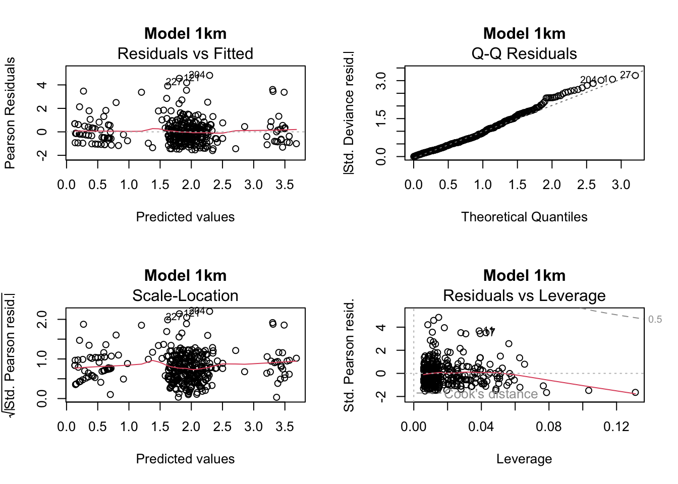
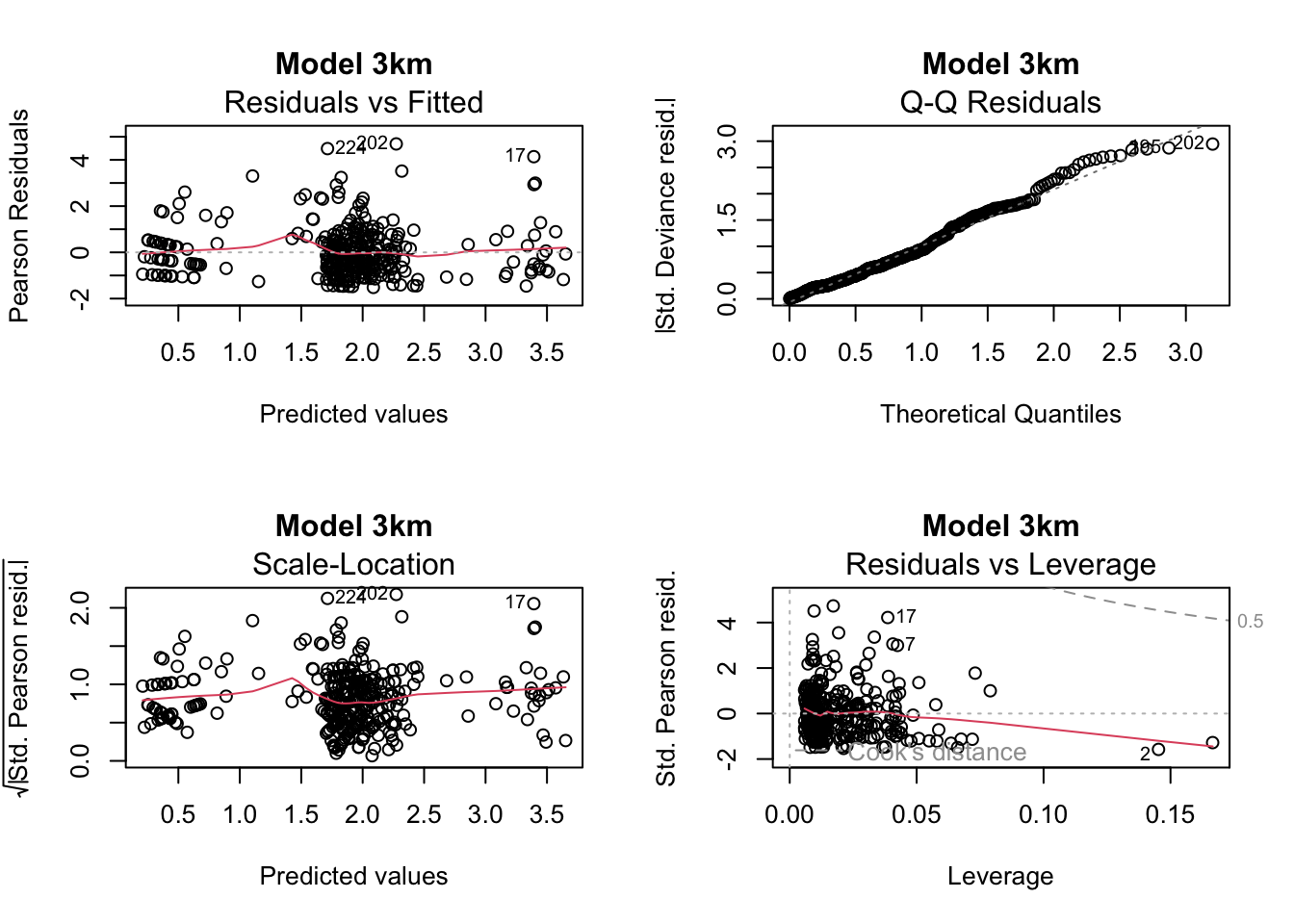
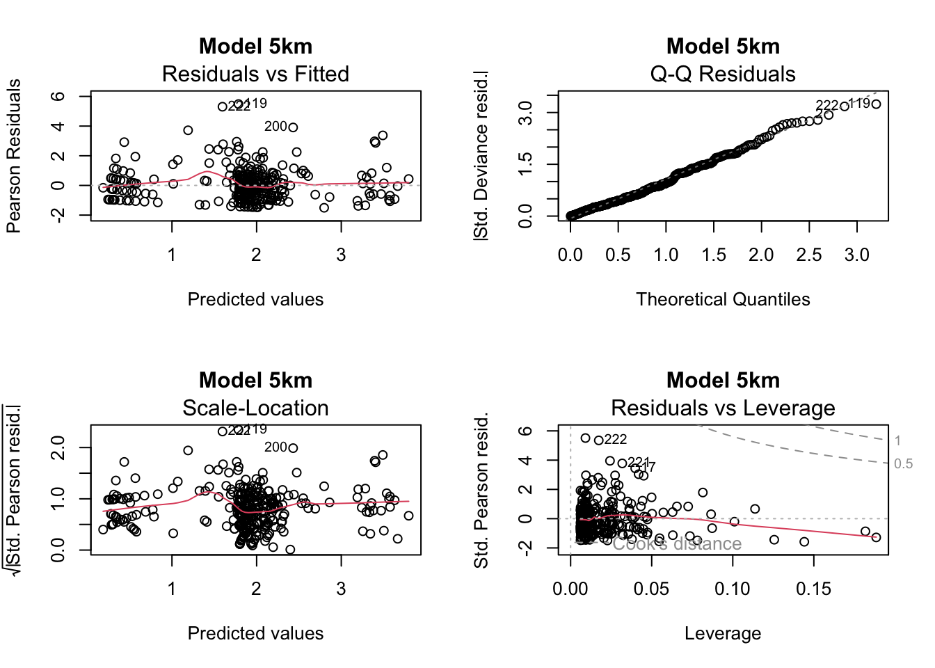
Basic diagnostics of the model residuals

models_GLM <- list(total_1km_m4, total_3km_m4, total_5km_m4)
model_names <- c("1km", "3km", "5km")

# Plot diagnostics
par(mfrow = c(2, 2))
for (i in 1:length(models_GLM)) {
  plot(models_GLM[[i]], main = paste("Model", model_names[i]))
}

par(mfrow = c(1, 1))

chat_values <- sapply(models_GLM, function(m) deviance(m) / df.residual(m))
names(chat_values) <- model_names
chat_values

     1km      3km      5km 
1.085849 1.093804 1.104432

Advanced diagnostics of the model residuals

simulationOutput <- simulateResiduals(fittedModel = total_1km_m4, plot = TRUE)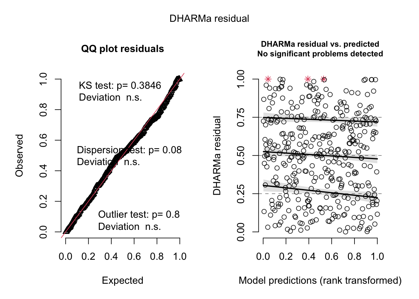

simulationOutput <- simulateResiduals(fittedModel = total_3km_m3, plot = TRUE)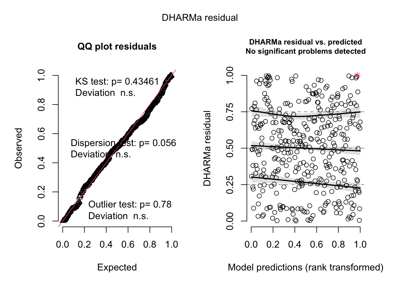

simulationOutput <- simulateResiduals(fittedModel = total_5km_m3, plot = TRUE)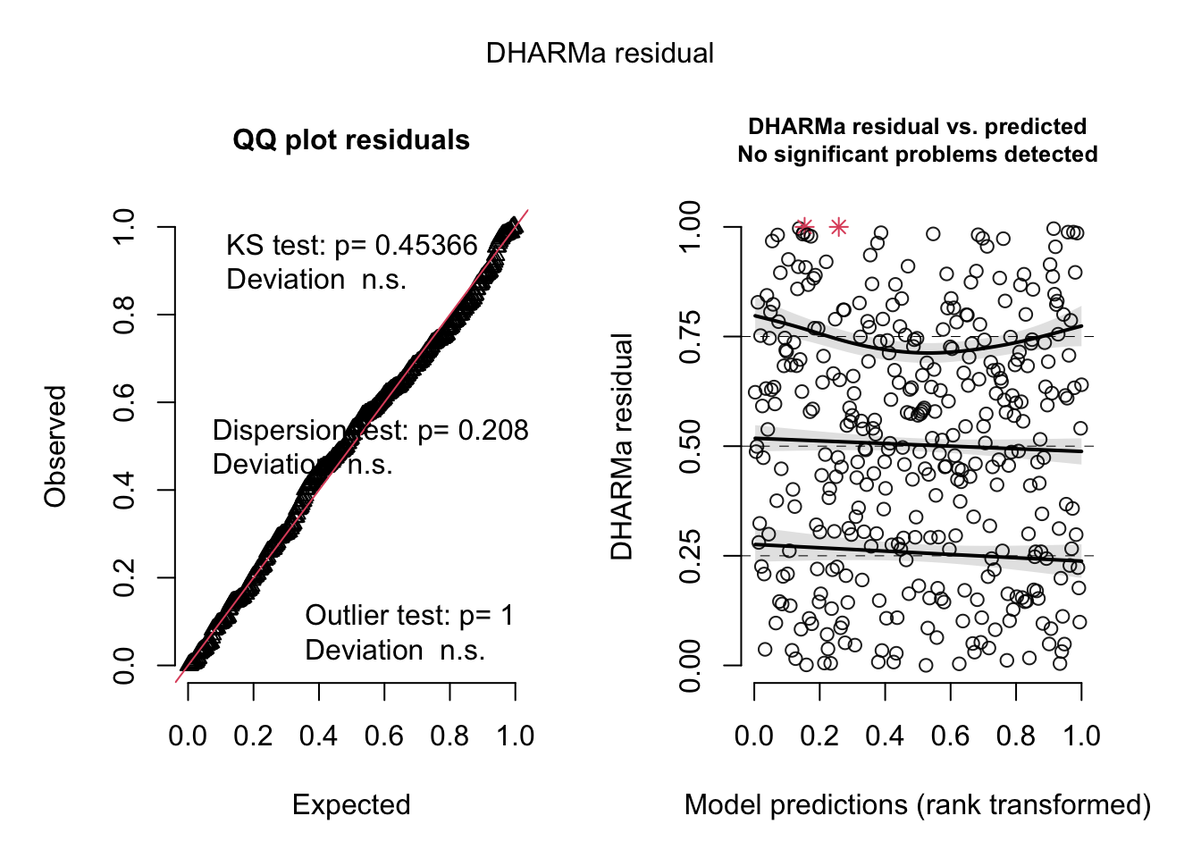

Summary

summary(total_1km_m4)


Call:
glm.nb(formula = total_roadkill_count ~ traffic + pavement + 
    urban_area + cult_land + savanna, data = d1km_sum, init.theta = 3.355735941, 
    link = log)

Coefficients:
            Estimate Std. Error z value Pr(>|z|)    
(Intercept)  0.86169    0.14849   5.803 6.51e-09 ***
traffic.L    1.12918    0.09128  12.371  < 2e-16 ***
traffic.Q    0.57746    0.07199   8.022 1.04e-15 ***
pavement1    1.53093    0.15134  10.116  < 2e-16 ***
urban_area  -0.28056    0.04263  -6.581 4.67e-11 ***
cult_land   -0.09536    0.04503  -2.118   0.0342 *  
savanna     -0.20642    0.04537  -4.550 5.36e-06 ***
---
Signif. codes:  0 '***' 0.001 '**' 0.01 '*' 0.05 '.' 0.1 ' ' 1

(Dispersion parameter for Negative Binomial(3.3557) family taken to be 1)

    Null deviance: 803.81  on 369  degrees of freedom
Residual deviance: 394.16  on 363  degrees of freedom
AIC: 2050.5

Number of Fisher Scoring iterations: 1

              Theta:  3.356 
          Std. Err.:  0.379 

 2 x log-likelihood:  -2034.463

summary(total_3km_m3)


Call:
glm.nb(formula = total_roadkill_count ~ traffic + pavement + 
    savanna + urban_area + forest + road_length, data = d3km_sum, 
    init.theta = 3.265092846, link = log)

Coefficients:
            Estimate Std. Error z value Pr(>|z|)    
(Intercept)  0.87078    0.15066   5.780 7.48e-09 ***
traffic.L    1.12092    0.09388  11.940  < 2e-16 ***
traffic.Q    0.56971    0.06930   8.221  < 2e-16 ***
pavement1    1.52605    0.15196  10.042  < 2e-16 ***
savanna     -0.08495    0.03855  -2.203   0.0276 *  
urban_area  -0.25050    0.04228  -5.925 3.13e-09 ***
forest       0.09023    0.03946   2.286   0.0222 *  
road_length  0.06654    0.03580   1.858   0.0631 .  
---
Signif. codes:  0 '***' 0.001 '**' 0.01 '*' 0.05 '.' 0.1 ' ' 1

(Dispersion parameter for Negative Binomial(3.2651) family taken to be 1)

    Null deviance: 784.85  on 366  degrees of freedom
Residual deviance: 393.38  on 359  degrees of freedom
AIC: 2046.1

Number of Fisher Scoring iterations: 1

              Theta:  3.265 
          Std. Err.:  0.366 

 2 x log-likelihood:  -2028.137

summary(total_5km_m3)


Call:
glm.nb(formula = total_roadkill_count ~ traffic + pavement + 
    road_length + forest + urban_area + savanna, data = d5km_sum, 
    init.theta = 3.104198301, link = log)

Coefficients:
            Estimate Std. Error z value Pr(>|z|)    
(Intercept)  0.87255    0.14938   5.841 5.18e-09 ***
traffic.L    1.13982    0.09825  11.602  < 2e-16 ***
traffic.Q    0.60949    0.07197   8.469  < 2e-16 ***
pavement1    1.55440    0.15158  10.255  < 2e-16 ***
road_length  0.10774    0.03614   2.981  0.00287 ** 
forest       0.10312    0.04218   2.445  0.01449 *  
urban_area  -0.22852    0.04187  -5.458 4.81e-08 ***
savanna     -0.07022    0.04074  -1.724  0.08478 .  
---
Signif. codes:  0 '***' 0.001 '**' 0.01 '*' 0.05 '.' 0.1 ' ' 1

(Dispersion parameter for Negative Binomial(3.1042) family taken to be 1)

    Null deviance: 777.05  on 363  degrees of freedom
Residual deviance: 395.17  on 356  degrees of freedom
AIC: 2041.2

Number of Fisher Scoring iterations: 1

              Theta:  3.104 
          Std. Err.:  0.347 

 2 x log-likelihood:  -2023.202

summary_1km_sum <- summary(total_1km_m4)
summary_3km_sum <- summary(total_3km_m3)
summary_5km_sum <- summary(total_5km_m3)

extract_est_p <- function(model_summary) {
  coef_table <- model_summary$coefficients
  data.frame(
    Term = rownames(coef_table),
    Estimate = coef_table[, "Estimate"],
    P_value = coef_table[, "Pr(>|z|)"],
    row.names = NULL
  )
}

df_1km_sum <- extract_est_p(summary_1km_sum)
df_3km_sum <- extract_est_p(summary_3km_sum)
df_5km_sum <- extract_est_p(summary_5km_sum)


GLM_scale_comparison <- df_1km_sum %>%
  rename(Estimate_1km = Estimate, P_1km = P_value) %>%
  full_join(df_3km_sum %>% rename(Estimate_3km = Estimate, P_3km = P_value), by = "Term") %>%
  full_join(df_5km_sum %>% rename(Estimate_5km = Estimate, P_5km = P_value), by = "Term")

GLM_scale_comparison

         Term Estimate_1km        P_1km Estimate_3km        P_3km Estimate_5km
1 (Intercept)   0.86168734 6.508918e-09   0.87077551 7.479045e-09   0.87255259
2   traffic.L   1.12918212 3.759111e-35   1.12092292 7.283471e-33   1.13981993
3   traffic.Q   0.57746179 1.040993e-15   0.56971078 2.026428e-16   0.60949099
4   pavement1   1.53092983 4.703616e-24   1.52604883 9.930132e-24   1.55439711
5  urban_area  -0.28055794 4.673442e-11  -0.25049720 3.126391e-09  -0.22852355
6   cult_land  -0.09536195 3.419241e-02           NA           NA           NA
7     savanna  -0.20642276 5.362968e-06  -0.08494518 2.756818e-02  -0.07022248
8      forest           NA           NA   0.09022897 2.223214e-02   0.10312374
9 road_length           NA           NA   0.06654221 6.310264e-02   0.10773605
         P_5km
1 5.182618e-09
2 4.044971e-31
3 2.477029e-17
4 1.127837e-24
5 4.814821e-08
6           NA
7 8.477630e-02
8 1.448584e-02
9 2.872694e-03

Plots

1km

Let’s assess which is the best set of graphs to represent the results found

Raw data

Pavement and traffic

The pavement and traffic plots are the same across all scales, so we will generate them only once using the 1 km dataset.

plot_pav <- d1km_raw_sum |> 
  ggplot(aes(x = factor(pavement), y = total_roadkill_count, fill = factor(pavement))) + 
  geom_boxplot(alpha = 0.5) +  
  scale_fill_manual(
    values = c("0" = "darkgoldenrod3", "1" = "gray40"),  
    labels = c("Unpaved", "Paved")
  ) +  
  scale_x_discrete(labels = c("0" = "Unpaved", "1" = "Paved")) +
  theme(
    panel.background = element_blank(),   
    axis.ticks = element_line(),          
    axis.title.x = element_text(size = 12), 
    axis.title.y = element_text(size = 12), 
    axis.text = element_text(size = 10),   
    axis.line = element_line()             
  ) +
  labs(
    x = "Pavement",         
    y = "Roadkill Number",
    fill = "Pavement"
  )

d1km_raw_sum$traffic <- factor(d1km_raw_sum$traffic, levels = c("low", "medium", "high"), ordered = TRUE)

plot_traffic <- d1km_raw_sum|> 
  ggplot(aes(x = factor(traffic), y = total_roadkill_count, fill = factor(traffic))) + 
  geom_boxplot(alpha = 0.5) +  
  scale_fill_manual(
    values = c("low" = "#FFDDC1", "medium" = "#FFD700", "high" = "#E63946"),  
    labels = c("Low", "Medium", "High")
  ) +  
  scale_x_discrete(labels = c("low" = "Low", "medium" = "Medium", "high" = "High")) +
  theme(
    panel.background = element_blank(),   
    axis.ticks = element_line(),          
    axis.title.x = element_text(size = 12), 
    axis.title.y = element_text(size = 12), 
    axis.text = element_text(size = 10),   
    axis.line = element_line()             
  ) +
  labs(
    x = "Traffic Level",         
    y = "Roadkill Number",
    fill = "Traffic Level"
  )

Urban area, cultivated land, and savanna

all appear to have a negative effect on roadkill numbers, according to the summar

vars <- c("urban_area", "savanna", "cult_land")
labels <- c("Urban Area (km²)", "Savanna Area (km²)", "Cultivated Land (km²)")

make_plot <- function(var, label_x) {
  ggplot(d1km_raw_sum, aes_string(x = var, y = "total_roadkill_count")) +
    geom_point(alpha = 1) +
    geom_smooth(method = "glm.nb", formula = y ~ x, se = TRUE, color = "red") +
    labs(x = label_x, y = "Roadkill Number") +
    theme(
      panel.background = element_blank(),
      axis.ticks = element_line(),
      axis.title = element_text(size = 12),
      axis.text = element_text(size = 10),
      axis.line = element_line()
    )
}

plots <- map2(vars, labels, make_plot)

Warning: `aes_string()` was deprecated in ggplot2 3.0.0.
ℹ Please use tidy evaluation idioms with `aes()`.
ℹ See also `vignette("ggplot2-in-packages")` for more information.

final_plot <- 
  (plot_pav | plot_traffic | patchwork::plot_spacer()) /
  (plots[[1]] | plots[[2]] | plots[[3]])

# Mostra o painel
final_plot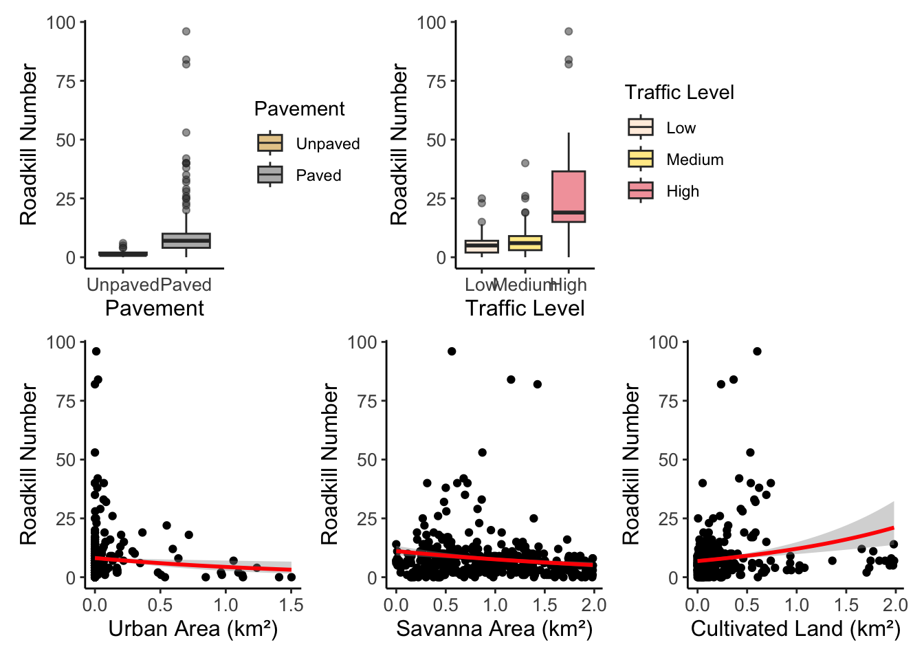

However, when plotting the raw data, cultivated land appears to have a positive effect.

Transformed data

Pavement and traffic

plot_pav_t <- d1km_raw_sum |> 
  ggplot(aes(x = factor(pavement), y = total_roadkill_count, fill = factor(pavement))) + 
  geom_boxplot(alpha = 0.5) +
  scale_y_continuous(trans = 'log10') +
  scale_fill_manual(
    values = c("0" = "darkgoldenrod3", "1" = "gray40"),  
    labels = c("Unpaved", "Paved")
  ) +  
  scale_x_discrete(labels = c("0" = "Unpaved", "1" = "Paved")) +
  theme(
    panel.background = element_blank(),   
    axis.ticks = element_line(),          
    axis.title.x = element_text(size = 12), 
    axis.title.y = element_text(size = 12), 
    axis.text = element_text(size = 10),   
    axis.line = element_line()             
  ) +
  labs(
    x = "Pavement",         
    y = "Roadkill Number",
    fill = "Pavement"
  )

plot_traffic_t <- d1km_raw_sum|> 
  ggplot(aes(x = factor(traffic), y = total_roadkill_count, fill = factor(traffic))) + 
  geom_boxplot(alpha = 0.5) +
  scale_y_continuous(trans = 'log10') +
  scale_fill_manual(
    values = c("low" = "#FFDDC1", "medium" = "#FFD700", "high" = "#E63946"),  
    labels = c("Low", "Medium", "High")
  ) +  
  scale_x_discrete(labels = c("low" = "Low", "medium" = "Medium", "high" = "High")) +
  theme(
    panel.background = element_blank(),   
    axis.ticks = element_line(),          
    axis.title.x = element_text(size = 12), 
    axis.title.y = element_text(size = 12), 
    axis.text = element_text(size = 10),   
    axis.line = element_line()             
  ) +
  labs(
    x = "Traffic Level",         
    y = "Roadkill Number",
    fill = "Traffic Level"
  )

Urban area, cultivated land, and savanna (log10)

make_plot_t <- function(var, label_x) {
  ggplot(d1km_sum, aes_string(x = var, y = "total_roadkill_count")) +
    geom_point(alpha = 1) +
    geom_smooth(method = "glm.nb", formula = y ~ x, se = TRUE, color = "red") +
    labs(x = label_x, y = "Roadkill Number") +
    theme(
      panel.background = element_blank(),
      axis.ticks = element_line(),
      axis.title = element_text(size = 12),
      axis.text = element_text(size = 10),
      axis.line = element_line()
    )
}

plots_t <- map2(vars, labels, make_plot_t)

final_plot_t <- 
  (plot_pav_t | plot_traffic_t | patchwork::plot_spacer()) /
  (plots_t[[1]] | plots_t[[2]] | plots_t[[3]])

final_plot_t

Warning in scale_y_continuous(trans = "log10"): log-10 transformation
introduced infinite values.

Warning: Removed 19 rows containing non-finite outside the scale range
(`stat_boxplot()`).

Warning in scale_y_continuous(trans = "log10"): log-10 transformation
introduced infinite values.

Warning: Removed 19 rows containing non-finite outside the scale range
(`stat_boxplot()`).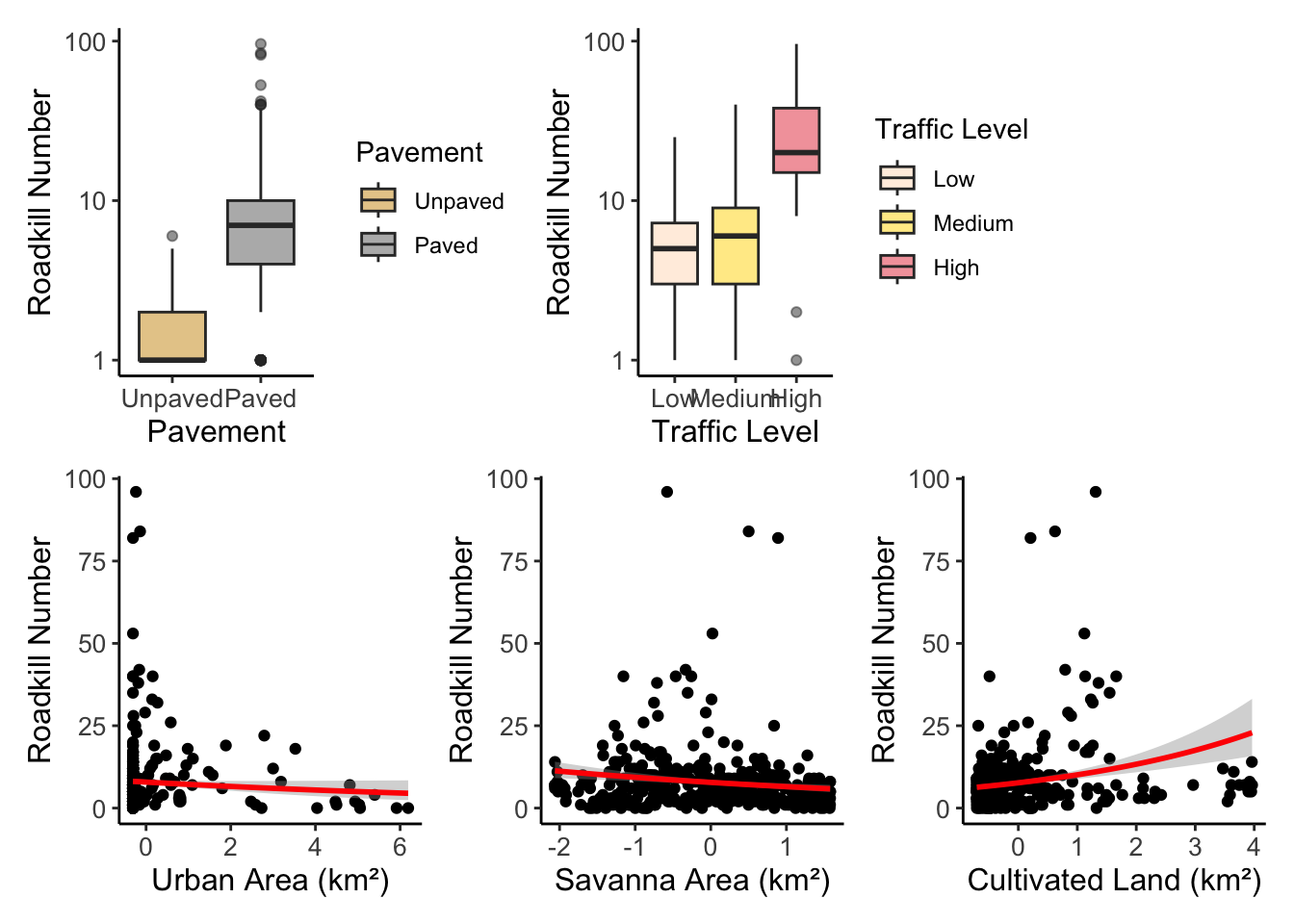

Model-predicted responses to environmental variables

landscape_vars_1km <- c("cult_land", "savanna", "urban_area")
landscape_plots <- list()  

for (var in landscape_vars_1km) {
  landscape_effect <- ggpredict(total_1km_m4, terms = var, bias_correction = TRUE)
  
  
  x_label <- paste("log10 of", var, "(km²)")
  
  plot_predict <- ggplot(landscape_effect, aes(x = x, y = predicted)) +
    geom_point(size = 3, color = "#FFD700") +
    geom_line(color = "#FFD700") +
    labs(title = paste("Effect of", var, "on Roadkill number"),
         x = x_label, 
         y = "Predicted roadkill") +
    theme_minimal()
  
  landscape_plots[[var]] <- plot_predict
}

Bias-correction is currently only supported for mixed or gee models. No
  bias-correction is applied.
Bias-correction is currently only supported for mixed or gee models. No
  bias-correction is applied.
Bias-correction is currently only supported for mixed or gee models. No
  bias-correction is applied.

final_plot_predict_1km <- (plot_pav_t | plot_traffic_t) / 
              (landscape_plots$cult_land | landscape_plots$savanna | landscape_plots$urban_area)

final_plot_predict_1km

Warning in scale_y_continuous(trans = "log10"): log-10 transformation
introduced infinite values.

Warning: Removed 19 rows containing non-finite outside the scale range
(`stat_boxplot()`).

Warning in scale_y_continuous(trans = "log10"): log-10 transformation
introduced infinite values.

Warning: Removed 19 rows containing non-finite outside the scale range
(`stat_boxplot()`).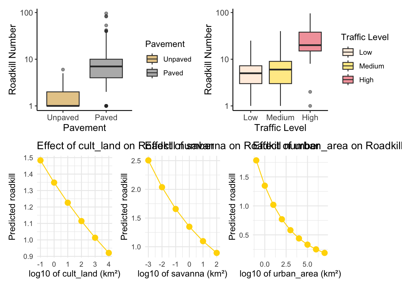

I believe that the graph with the model’s prediction looks better, although it is a bit harder to interpret. However, since the other graphs show the relationship between the proportion of cultivated land and the number of roadkills in an opposite relationship to what is shown in the model’s summary, let’s use only this set of graphs for the other scales

3km

Model-predicted responses to environmental variables

landscape_vars_3km <- c("road_length", "savanna", "urban_area", "forest" )
landscape_plots <- list()  

for (var in landscape_vars_3km) {
  landscape_effect <- ggpredict(total_3km_m3, terms = var, bias_correction = TRUE)
  
  
  x_label <- paste("log10 of", var, "(km²)")
  
  plot_predict <- ggplot(landscape_effect, aes(x = x, y = predicted)) +
    geom_point(size = 3, color = "#1f77b4") +
    geom_line(color = "#1f77b4") +
    labs(x = x_label, 
         y = "Predicted roadkill") +
    theme_minimal()
  
  landscape_plots[[var]] <- plot_predict
}

Bias-correction is currently only supported for mixed or gee models. No
  bias-correction is applied.
Bias-correction is currently only supported for mixed or gee models. No
  bias-correction is applied.
Bias-correction is currently only supported for mixed or gee models. No
  bias-correction is applied.
Bias-correction is currently only supported for mixed or gee models. No
  bias-correction is applied.

final_plot_predict_3km <- (plot_pav_t | plot_traffic_t) / 
              (landscape_plots$road_length | landscape_plots$savanna |landscape_plots$fores | landscape_plots$urban_area)

final_plot_predict_3km

Warning in scale_y_continuous(trans = "log10"): log-10 transformation
introduced infinite values.

Warning: Removed 19 rows containing non-finite outside the scale range
(`stat_boxplot()`).

Warning in scale_y_continuous(trans = "log10"): log-10 transformation
introduced infinite values.

Warning: Removed 19 rows containing non-finite outside the scale range
(`stat_boxplot()`).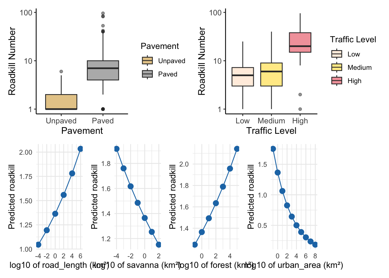

5km

Model-predicted responses to environmental variables

landscape_vars_5km <- c("road_length", "savanna", "urban_area", "forest" )
landscape_plots <- list()  

for (var in landscape_vars_5km) {
  landscape_effect <- ggpredict(total_5km_m3, terms = var, bias_correction = TRUE)
  
  
  x_label <- paste("log10 of", var, "(km²)")
  
  plot_predict <- ggplot(landscape_effect, aes(x = x, y = predicted)) +
    geom_point(size = 3, color = "#9B59B6") +
    geom_line(color = "#9B59B6") +
    labs(x = x_label, 
         y = "Predicted roadkill") +
    theme_minimal()
  
  landscape_plots[[var]] <- plot_predict
}

Bias-correction is currently only supported for mixed or gee models. No
  bias-correction is applied.
Bias-correction is currently only supported for mixed or gee models. No
  bias-correction is applied.
Bias-correction is currently only supported for mixed or gee models. No
  bias-correction is applied.
Bias-correction is currently only supported for mixed or gee models. No
  bias-correction is applied.

final_plot_predict_5km <- (plot_pav_t | plot_traffic_t) / 
              (landscape_plots$road_length | landscape_plots$savanna |landscape_plots$fores | landscape_plots$urban_area)

final_plot_predict_5km

Warning in scale_y_continuous(trans = "log10"): log-10 transformation
introduced infinite values.

Warning: Removed 19 rows containing non-finite outside the scale range
(`stat_boxplot()`).

Warning in scale_y_continuous(trans = "log10"): log-10 transformation
introduced infinite values.

Warning: Removed 19 rows containing non-finite outside the scale range
(`stat_boxplot()`).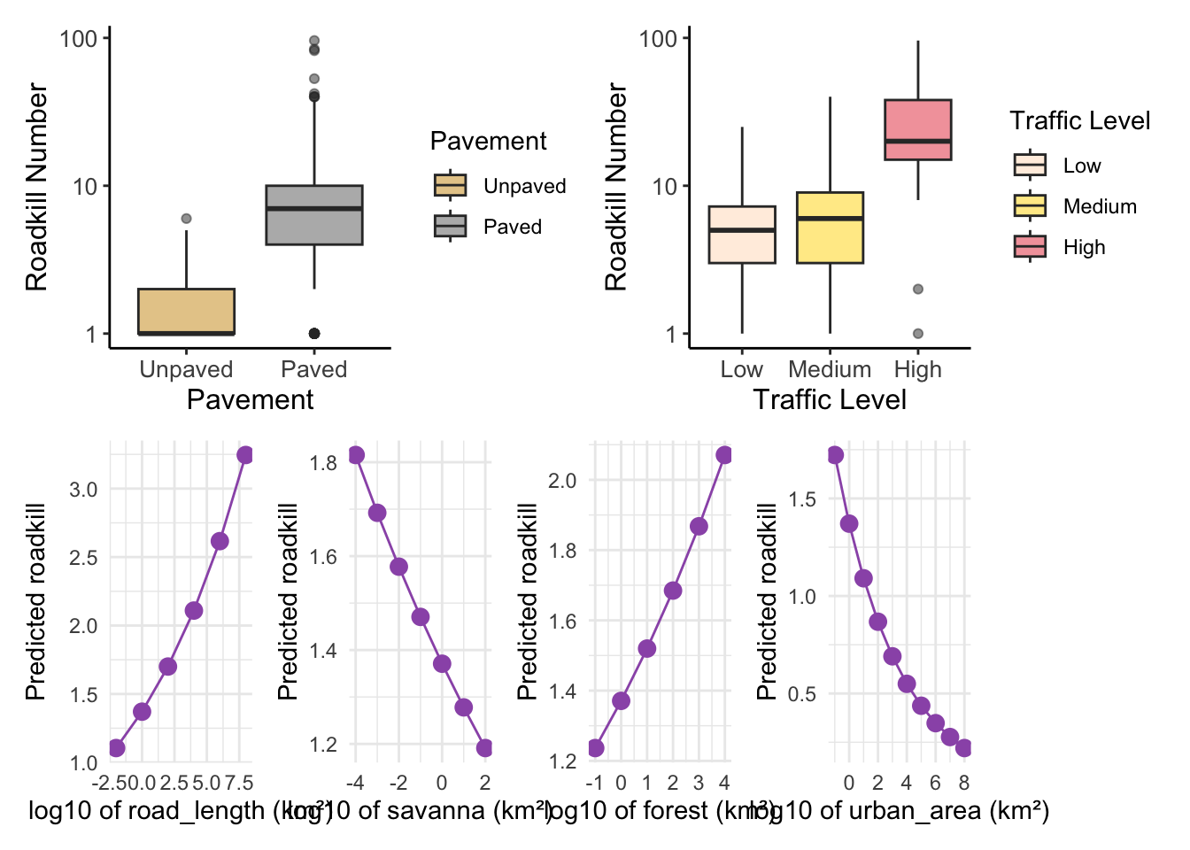

Number of roadkill: taxa and sazonality

GLMM - Negative binomial

format_data_GLMM <- function(df) {
  df$polygon <- as.factor(df$polygon)
  df$pavement <- factor(df$pavement, levels = c("0", "1"))
  df$traffic <- factor(df$traffic, levels = c("low", "medium", "high"), ordered = TRUE)
  df$taxa <- factor(df$taxa, levels = c("amp","rep", "bird", "mam"))
  df$season <- factor(df$season, levels = c("dry","rainy"))
  df$water <- as.numeric(df$water)
  df$road_length <- as.numeric(df$road_length)
  df$shrubby <- as.numeric(df$shrubby)
  df$urban_area <- as.numeric(df$urban_area)
  df$cult_land <- as.numeric(df$cult_land)
  df$savanna <- as.numeric(df$savanna)
  df$forest <- as.numeric(df$forest)
  df$p <- as.numeric(df$savanna)
  return(df)
}

d1km <- format_data_GLMM(d1km)
d3km <- format_data_GLMM(d3km)
d5km <- format_data_GLMM(d5km)

1km

taxa_1km_m0 <- glmmTMB(roadkill_count ~ pavement * taxa + traffic + season + cult_land + urban_area + forest + savanna + water + shrubby + road_length + (1 | polygon),
                     family = nbinom2,
                        data = d1km)

3km

taxa_3km_m0 <- glmmTMB(roadkill_count ~ pavement * taxa + traffic + season + cult_land + urban_area + forest + savanna + water + shrubby + road_length + (1 | polygon),
                     family = nbinom2,
                        data = d3km)

5km

taxa_5km_m0 <- glmmTMB(roadkill_count ~ pavement * taxa + traffic + season + cult_land + urban_area + forest + savanna + water + shrubby + road_length + (1 | polygon),
                     family = nbinom2,
                        data = d5km)

R² values

Calculation of Pseudo R² (Nagelkerke)

models_GLMM <- list(
  taxa_1km_m0 = taxa_1km_m0,
  taxa_3km_m0 = taxa_3km_m0,
  taxa_5km_m0 = taxa_5km_m0
)

r2_results <- lapply(models_GLMM, r2_nakagawa)

cat("\nPseudo R² of the models:\n")


Pseudo R² of the models:

print(r2_results)

$taxa_1km_m0
# R2 for Mixed Models

  Conditional R2: 0.447
     Marginal R2: 0.323

$taxa_3km_m0
# R2 for Mixed Models

  Conditional R2: 0.440
     Marginal R2: 0.310

$taxa_5km_m0
# R2 for Mixed Models

  Conditional R2: 0.449
     Marginal R2: 0.309

Advanced diagnostics of the model residuals

simulationOutput <- simulateResiduals(fittedModel = taxa_1km_m0, plot = TRUE)

DHARMa:testOutliers with type = binomial may have inflated Type I error rates for integer-valued distributions. To get a more exact result, it is recommended to re-run testOutliers with type = 'bootstrap'. See ?testOutliers for details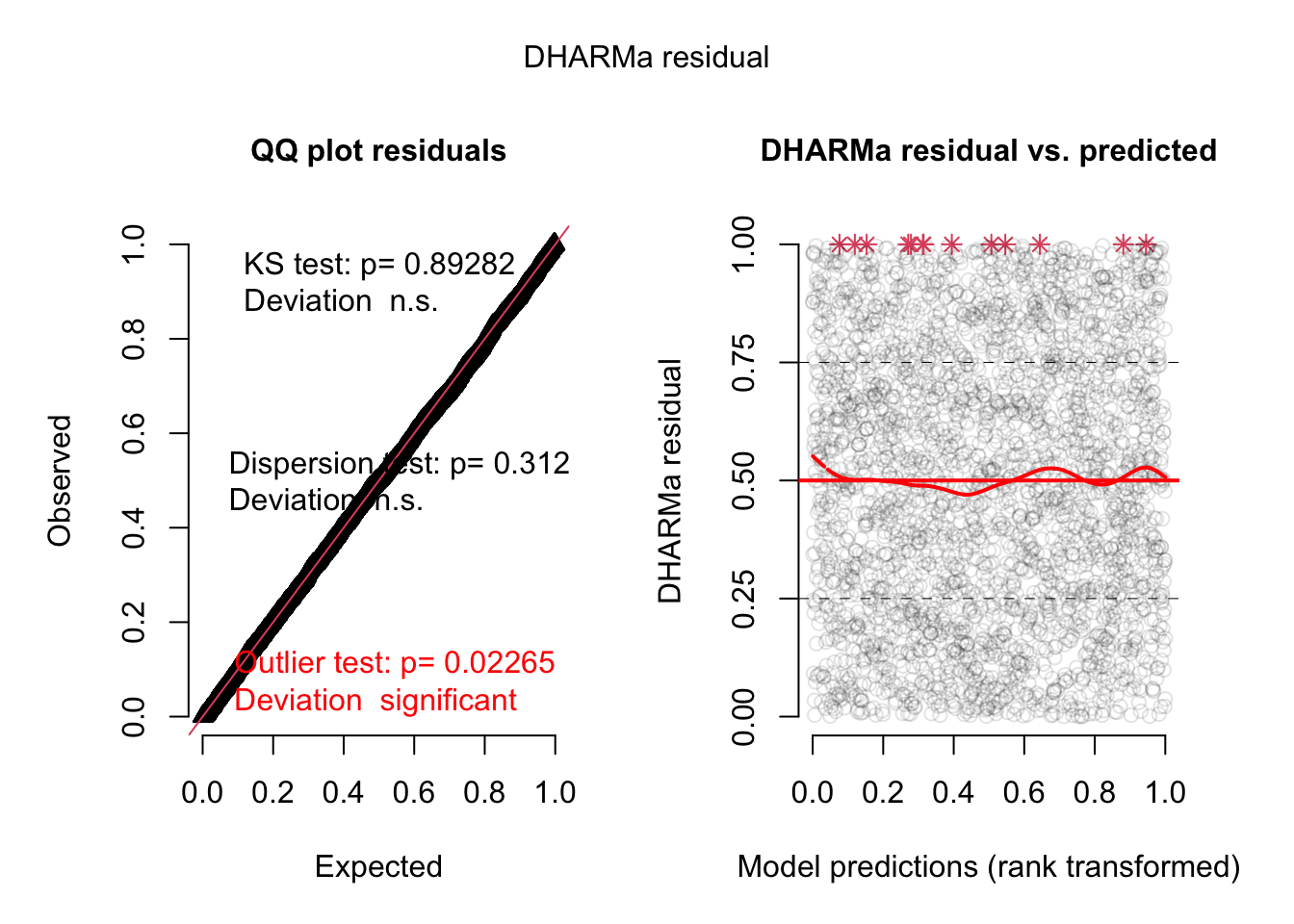

simulationOutput <- simulateResiduals(fittedModel = taxa_3km_m0, plot = TRUE)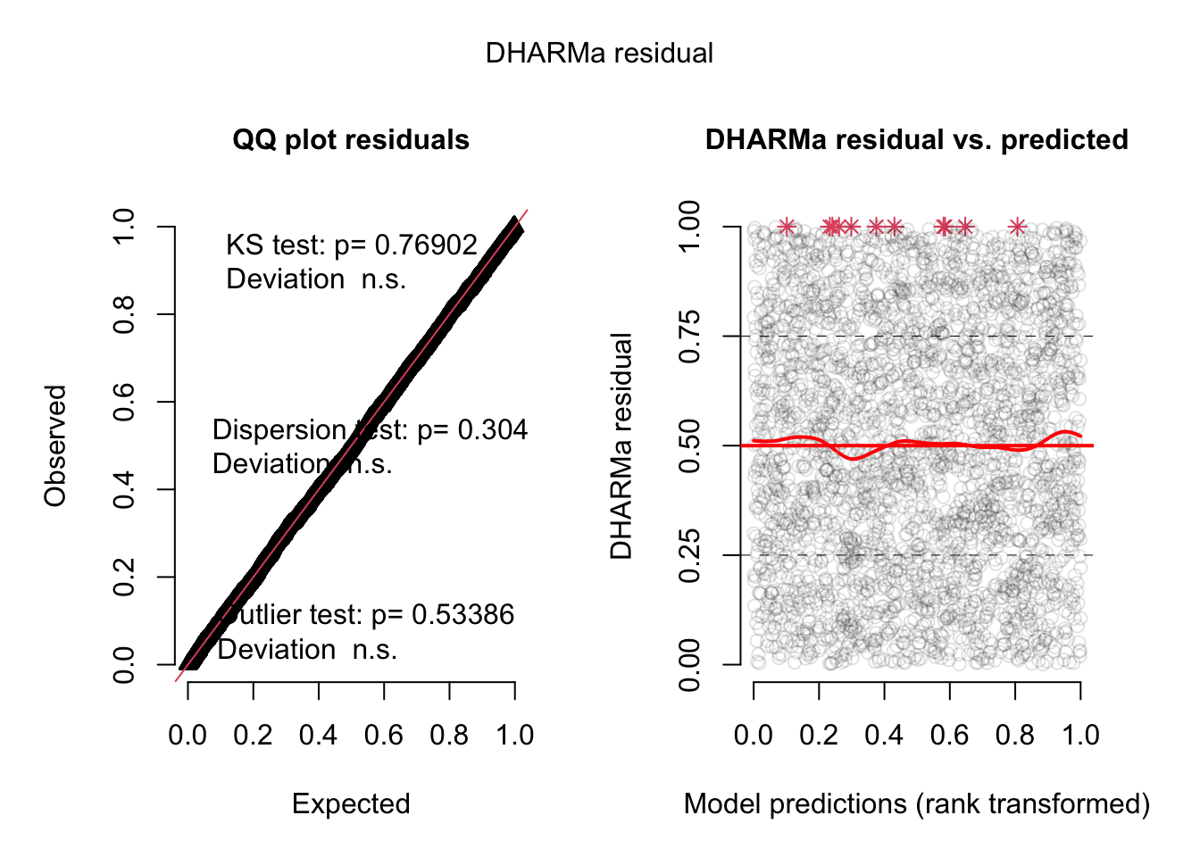

simulationOutput <- simulateResiduals(fittedModel = taxa_5km_m0, plot = TRUE)

DHARMa:testOutliers with type = binomial may have inflated Type I error rates for integer-valued distributions. To get a more exact result, it is recommended to re-run testOutliers with type = 'bootstrap'. See ?testOutliers for details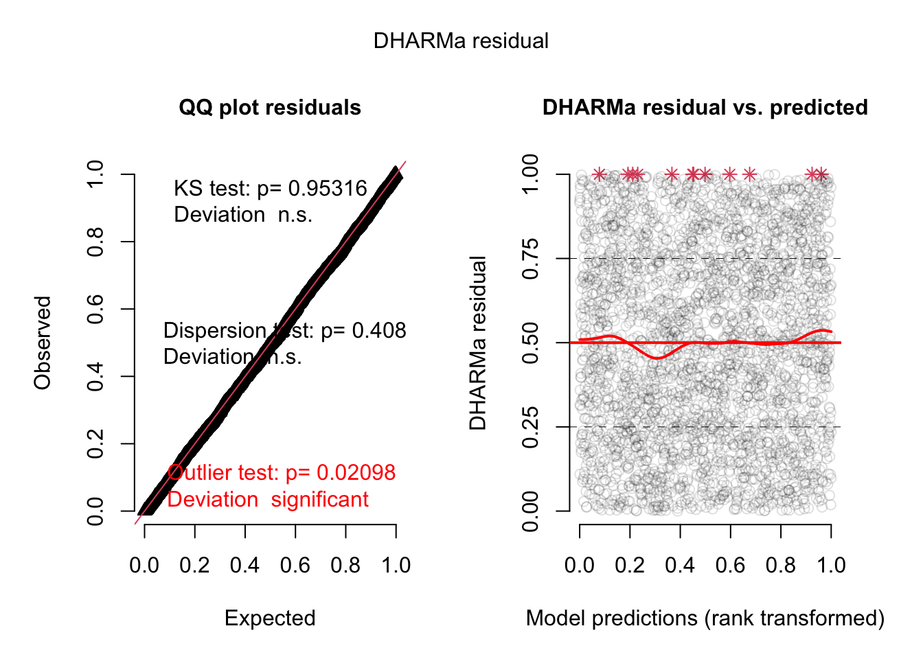

Since the outliers in the datasets are real data (and not errors) primarily related to seasonality, these data will be retained even if the model is not able to represent them very well.

Summary

# Function to extract estimates and p-values, adding an asterisk for significance
extract_est_p <- function(model_summary) {
  coef_table <- model_summary$coefficients$cond  # Accessing coefficients
  
  # Create the table with estimates and p-values
  result <- data.frame(
    Term = rownames(coef_table),
    Estimate = coef_table[, "Estimate"],
    P_value = coef_table[, "Pr(>|z|)"],
    row.names = NULL
  )
  
  # Add an asterisk to p-values that are significant (p < 0.05)
  result$P_value <- ifelse(result$P_value < 0.05, paste(result$P_value, "*", sep=""), result$P_value)
  
  return(result)
}

# Extract data for the three models
df_1km <- extract_est_p(summary(taxa_1km_m0))
df_3km <- extract_est_p(summary(taxa_3km_m0))
df_5km <- extract_est_p(summary(taxa_5km_m0))

# Comparison across scales
GLMM_scale_comparison <- df_1km %>%
  rename(Estimate_1km = Estimate, P_1km = P_value) %>%
  full_join(df_3km %>% rename(Estimate_3km = Estimate, P_3km = P_value), by = "Term") %>%
  full_join(df_5km %>% rename(Estimate_5km = Estimate, P_5km = P_value), by = "Term")

# Display the comparison table with asterisks for significant p-values
GLMM_scale_comparison

                 Term Estimate_1km                 P_1km Estimate_3km
1         (Intercept) -1.371464595 4.83666098700055e-08*  -1.31876922
2           pavement1  1.354032867 1.12729224666042e-07*   1.31929639
3             taxarep -0.142282009      0.67758325239058  -0.21859770
4            taxabird -0.028331463     0.932338006427453  -0.06222133
5             taxamam -0.443769275     0.232781562871888  -0.47113619
6           traffic.L  1.067004720 3.46285373264564e-31*   1.09207691
7           traffic.Q  0.527500873  1.5117181595587e-12*   0.54905749
8         seasonrainy  0.308423015 7.09611642478015e-10*   0.30483518
9           cult_land -0.070557293     0.123338540517713  -0.01101422
10         urban_area -0.316348347 1.65068806737414e-12*  -0.28628866
11             forest -0.006687915     0.859792649755936   0.07688007
12            savanna -0.184789440 8.61500679258319e-05*  -0.08768001
13              water  0.033410198     0.323308747498995   0.05289200
14            shrubby -0.071765224     0.114336543459419  -0.04119905
15        road_length  0.054259772     0.161619830151198   0.07477562
16  pavement1:taxarep -0.052613424     0.880572525219733   0.02023970
17 pavement1:taxabird  0.248596666     0.465993473159678   0.29044073
18  pavement1:taxamam  0.482259554     0.202847051107338   0.50900106
                   P_3km Estimate_5km                 P_5km
1  1.12405633695864e-07*  -1.27178523 1.64726508732981e-07*
2  1.82208116289844e-07*   1.26534756 3.15802212938161e-07*
3      0.526493571164108  -0.25438083     0.449796379677468
4      0.851321752891221  -0.19938198     0.547757201883857
5      0.203390364446111  -0.55350317     0.131067285049484
6  7.94836469897303e-28*   1.10525542 5.52372761087828e-25*
7  5.05976909759541e-13*   0.56652780 1.17734472819166e-12*
8  1.49011217183763e-09*   0.31617197 5.06407066605247e-10*
9      0.838252428594515   0.02034147     0.701605963705215
10 5.96583304385389e-10*  -0.26576535 6.04093577621799e-09*
11    0.0887220734848294   0.09968404   0.0480166694322663*
12      0.11056060987862  -0.06156999     0.264456094135544
13     0.146644306208703   0.06302950     0.106649367400041
14     0.310426500955283  -0.04617115     0.260074679852243
15   0.0351920677742152*   0.11974674 0.000931309455736103*
16     0.954293591278449   0.07967533     0.817333753926652
17     0.392164741011497   0.44716588     0.187535808111879
18     0.177331223067328   0.60234772     0.107005824547447

Plots

Pavement on Roadkill by Vertebrate Group

At none of the spatial scales was the p-value significant for the different taxa, not even when evaluating their interaction with pavement. Therefore, the plots are merely illustrative and should be interpreted with caution

plot_pav_taxa_effect <- function(model, titulo = "Pavement effect") {
  
  
  plot_data <- ggpredict(model, terms = c("pavement", "taxa"), bias_correction = TRUE)
  

  p <- ggplot(plot_data, aes(x = x, y = predicted, color = group)) +
    geom_point(size = 2) +
    geom_line(aes(group = group)) +
    geom_ribbon(aes(ymin = conf.low, ymax = conf.high, fill = group), alpha = 0.2, color = NA) +
    labs(
      title = titulo,
      x = "0 = unpaver, 1 = paved",
      y = "Predicted roadkill number",
      color = "Taxa",
      fill = "Taxa"
    ) +
    theme_bw() +
    theme(
      plot.title = element_text(hjust = 0.5),
      legend.position = "right"
    ) +
    scale_color_brewer(palette = "Dark2") +
    scale_fill_brewer(palette = "Dark2")
  
  return(p)
}

plot_pav_taxa_effect(taxa_1km_m0, "Pavement x Taxa (1 km)")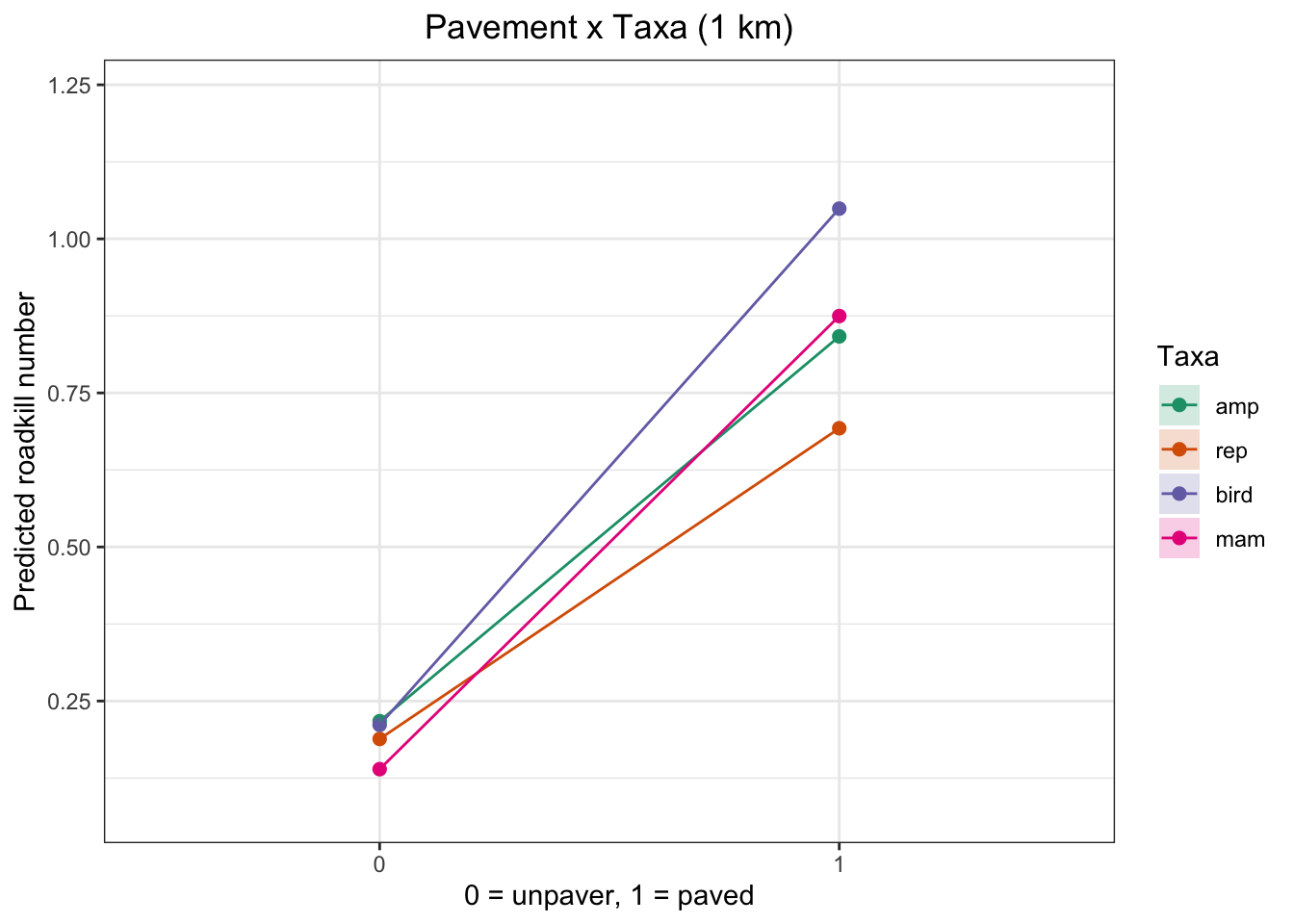

plot_pav_taxa_effect(taxa_3km_m0, "Pavement x Taxa (3 km)")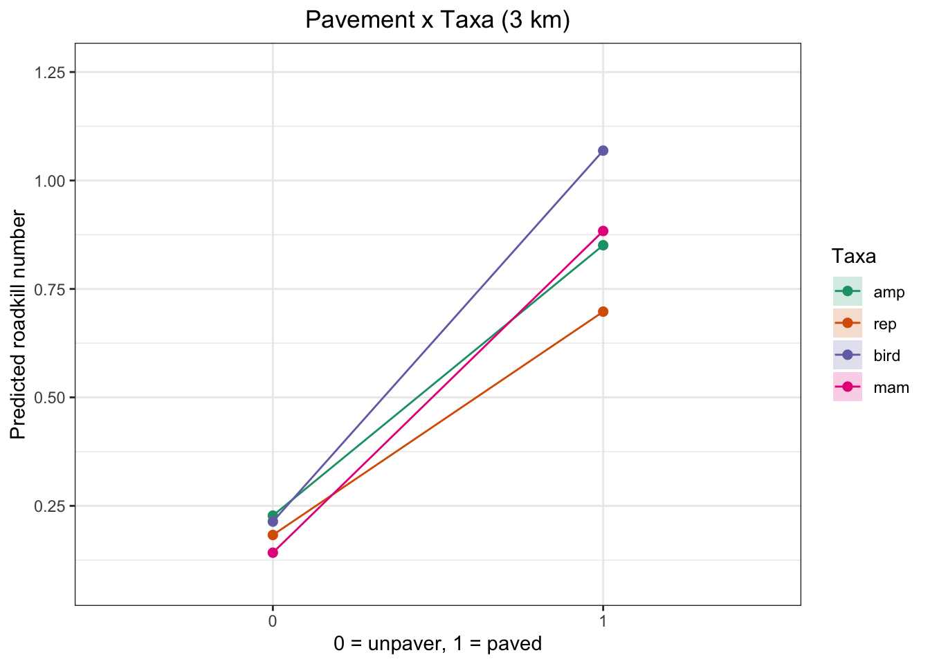

plot_pav_taxa_effect(taxa_5km_m0, "Pavement x Taxa (5 km)")

Traffic on Roadkill

traffic_1km <- ggpredict(taxa_1km_m0, terms = "traffic", bias_correction = TRUE) %>%
  mutate(Scale = "1km")

traffic_3km <- ggpredict(taxa_3km_m0, terms = "traffic", bias_correction = TRUE) %>%
  mutate(Scale = "3km")

traffic_5km <- ggpredict(taxa_5km_m0, terms = "traffic", bias_correction = TRUE) %>%
  mutate(Scale = "5km")


traffic_all <- bind_rows(traffic_1km, traffic_3km, traffic_5km) %>%
  filter(!is.na(x), !is.na(predicted))


ggplot(traffic_all, aes(x = x, y = predicted, fill = Scale)) +
  geom_col(position = position_dodge(width = 0.9), alpha = 0.7) +
  geom_errorbar(aes(ymin = conf.low, ymax = conf.high),
                position = position_dodge(width = 0.9), width = 0.2) +
  labs(title = "Effect of Traffic on Roadkill by Scale",
       x = "Traffic Level", 
       y = "Predicted Roadkill") +
  theme_bw() +
  scale_fill_manual(values = c("1km" = "#FFD700",  
                               "3km" = "#1f77b4",  
                               "5km" = "#9B59B6"))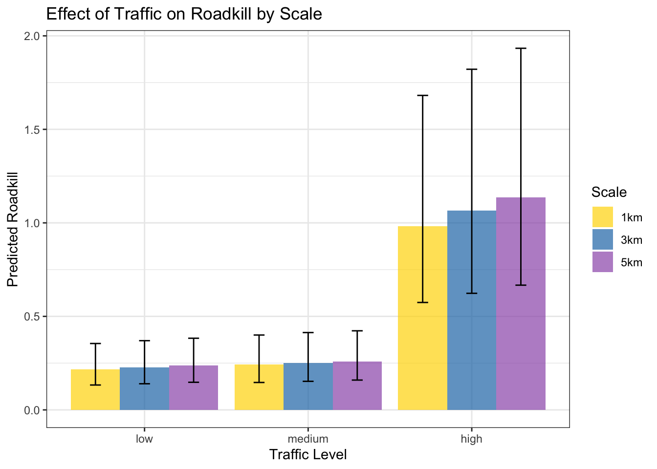

Seasonality and its effect on roadkilll

d1km$season <- factor(d1km$season, levels = c("dry", "rainy"))
d3km$season <- factor(d3km$season, levels = c("dry", "rainy"))
d5km$season <- factor(d5km$season, levels = c("dry", "rainy"))

season_1km <- ggpredict(taxa_1km_m0, terms = "season", bias_correction = TRUE) %>%
  mutate(Scale = "1km")

season_3km <- ggpredict(taxa_3km_m0, terms = "season", bias_correction = TRUE) %>%
  mutate(Scale = "3km")

season_5km <- ggpredict(taxa_5km_m0, terms = "season", bias_correction = TRUE) %>%
  mutate(Scale = "5km")

# Junta os dados
season_all <- bind_rows(season_1km, season_3km, season_5km)

# Remove possíveis NAs (opcional, por segurança)
season_all <- season_all %>% filter(!is.na(predicted))

# Gráfico
ggplot(season_all, aes(x = x, y = predicted, color = Scale, group = Scale)) +
  geom_point(position = position_dodge(width = 0.4), size = 3) +
  geom_line(position = position_dodge(width = 0.4)) +
  geom_errorbar(aes(ymin = conf.low, ymax = conf.high), 
                position = position_dodge(width = 0.4), width = 0.2) +
  labs(title = "Effect of Season on Roadkill by Scale",
       x = "Season", 
       y = "Predicted Roadkill") +
  scale_color_manual(values = c("1km" = "#FFD700",
                                "3km" = "#1f77b4",
                                "5km" = "#9B59B6")) +
  theme_bw()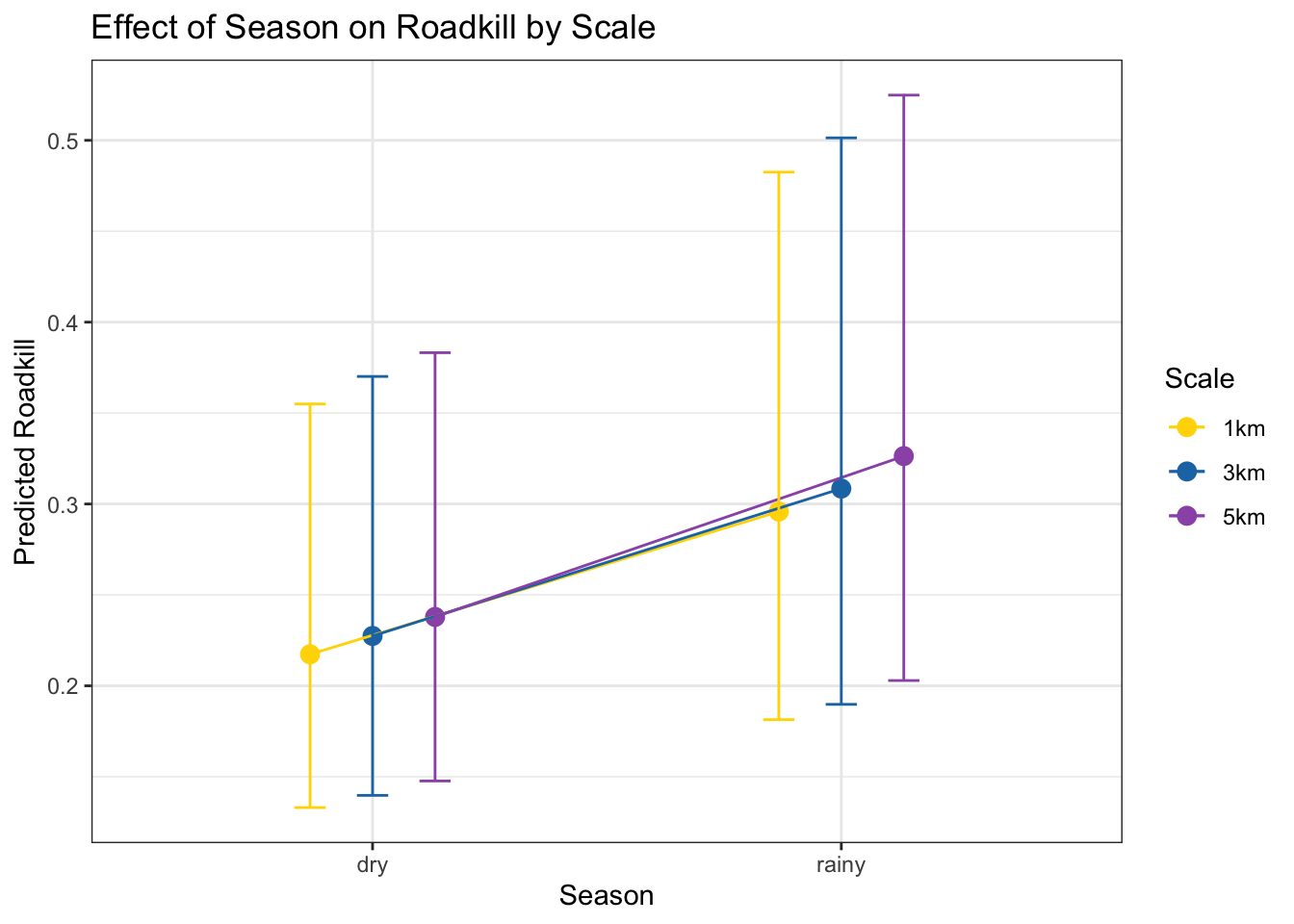

Landscape Variables on Roadkil

landscape_vars <- c("cult_land", "water", "shrubby", "urban_area", "forest", "savanna")
landscape_labels <- c("Cultivated land", "Water", "Shrubby", "Urban area", "Forest", "Savanna")


plot_list <- list()

for (i in 1:length(landscape_vars)) {
  var <- landscape_vars[i]
  label <- landscape_labels[i]
  
  landscape_effect <- ggpredict(taxa_1km_m0, terms = var, bias_correction = TRUE)
  
  p <- ggplot(landscape_effect, aes(x = x, y = predicted)) +
    geom_point(size = 2, color = "#FFD700") +
    geom_line(color = "black") +
    labs(x = label, y = NULL) +  
    scale_y_continuous(limits = c(0, 1)) +  
    theme_minimal() +
    theme(
      plot.title = element_blank(),
      panel.grid.major = element_blank(),  
      panel.grid.minor = element_blank(),  
      panel.border = element_blank(),      
      axis.line = element_line(color = "black"),  
      axis.text = element_text(size = 12),  
      axis.title.x = element_text(size = 14),  
      axis.title.y = element_text(size = 14),  
    )  
  
  plot_list[[var]] <- p
}


final_plot <- wrap_plots(plot_list, ncol = 3, byrow = TRUE) +  
  plot_annotation(title = NULL, tag_levels = NULL) & 
  theme(
    axis.title.y = element_text(angle = 90, vjust =0.5), 
    plot.margin = margin(10, 10, 10, 40)
  )

y_label <- ggdraw() + draw_label("Predicted Roadkill - 1km", angle = 90, hjust = 0.5)


plot_grid(y_label, final_plot, ncol = 2, rel_widths = c(0.05, 1))

3km

for (i in 1:length(landscape_vars)) {
  var <- landscape_vars[i]
  label <- landscape_labels[i]
  
  landscape_effect <- ggpredict(taxa_3km_m0, terms = var, bias_correction = TRUE)
  
  p <- ggplot(landscape_effect, aes(x = x, y = predicted)) +
    geom_point(size = 2, color = "#1f77b4") +
    geom_line(color = "black") +
    labs(x = label, y = NULL) +  
    scale_y_continuous(limits = c(0, 1)) +  
    theme_minimal() +
    theme(
      plot.title = element_blank(),
      panel.grid.major = element_blank(),  
      panel.grid.minor = element_blank(),  
      panel.border = element_blank(),      
      axis.line = element_line(color = "black"),  
      axis.text = element_text(size = 12),  
      axis.title.x = element_text(size = 14),  
      axis.title.y = element_text(size = 14),  
    )  
  
  plot_list[[var]] <- p
}


final_plot <- wrap_plots(plot_list, ncol = 3, byrow = TRUE) +  
  plot_annotation(title = NULL, tag_levels = NULL) & 
  theme(
    axis.title.y = element_text(angle = 90, vjust =0.5), 
    plot.margin = margin(10, 10, 10, 40)
  )

y_label <- ggdraw() + draw_label("Predicted Roadkill - 3km", angle = 90, hjust = 0.5)


plot_grid(y_label, final_plot, ncol = 2, rel_widths = c(0.05, 1))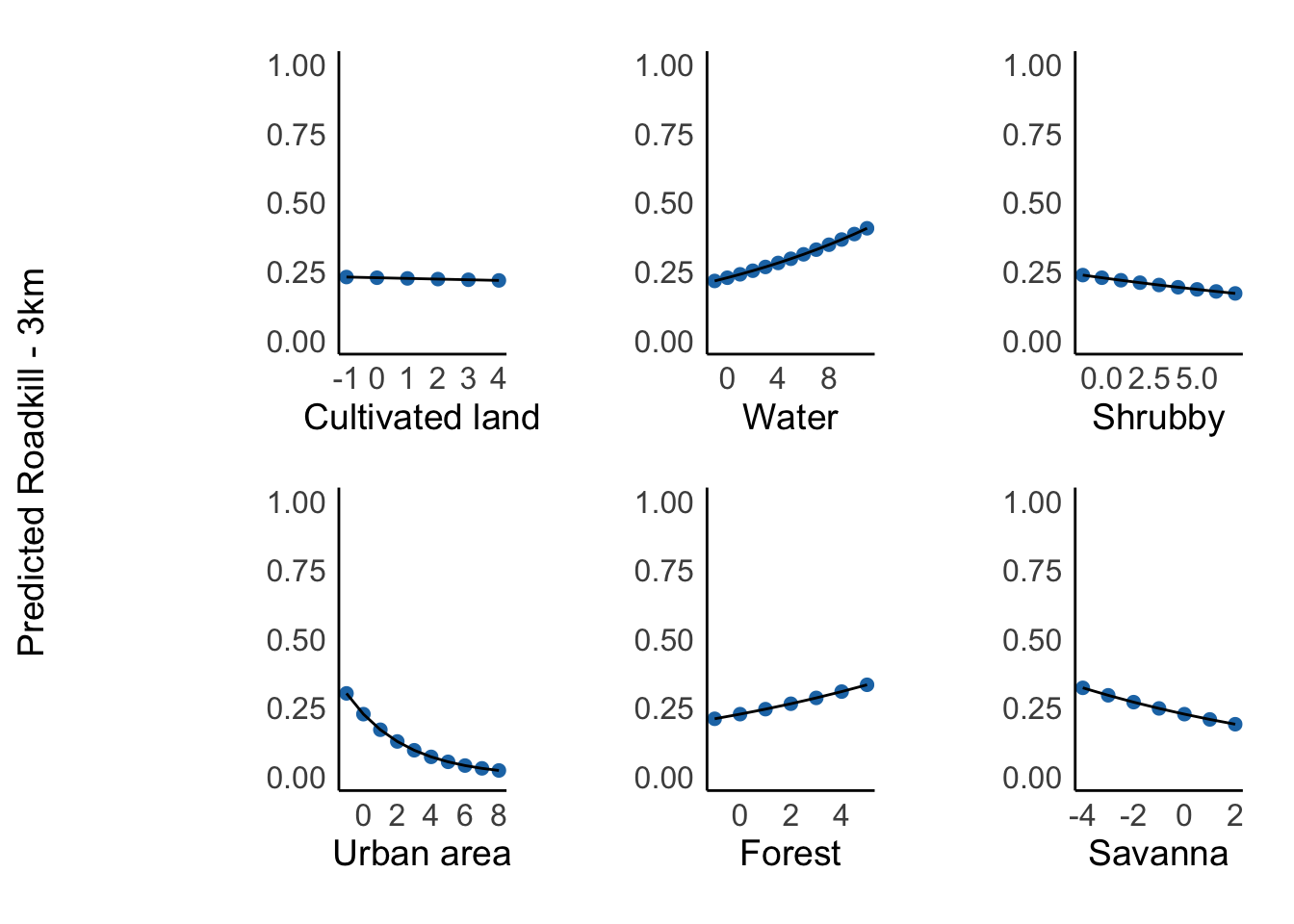

for (i in 1:length(landscape_vars)) {
  var <- landscape_vars[i]
  label <- landscape_labels[i]
  
  landscape_effect <- ggpredict(taxa_5km_m0, terms = var, bias_correction = TRUE)
  
  p <- ggplot(landscape_effect, aes(x = x, y = predicted)) +
    geom_point(size = 2, color = "#9B59B6") +
    geom_line(color = "black") +
    labs(x = label, y = NULL) +  
    scale_y_continuous(limits = c(0, 1)) +  
    theme_minimal() +
    theme(
      plot.title = element_blank(),
      panel.grid.major = element_blank(),  
      panel.grid.minor = element_blank(),  
      panel.border = element_blank(),      
      axis.line = element_line(color = "black"),  
      axis.text = element_text(size = 12),  
      axis.title.x = element_text(size = 14),  
      axis.title.y = element_text(size = 14),  
    )  
  
  plot_list[[var]] <- p
}


final_plot <- wrap_plots(plot_list, ncol = 3, byrow = TRUE) +  
  plot_annotation(title = NULL, tag_levels = NULL) & 
  theme(
    axis.title.y = element_text(angle = 90, vjust =0.5), 
    plot.margin = margin(10, 10, 10, 40)
  )

y_label <- ggdraw() + draw_label("Predicted Roadkill - 5km", angle = 90, hjust = 0.5)


plot_grid(y_label, final_plot, ncol = 2, rel_widths = c(0.05, 1))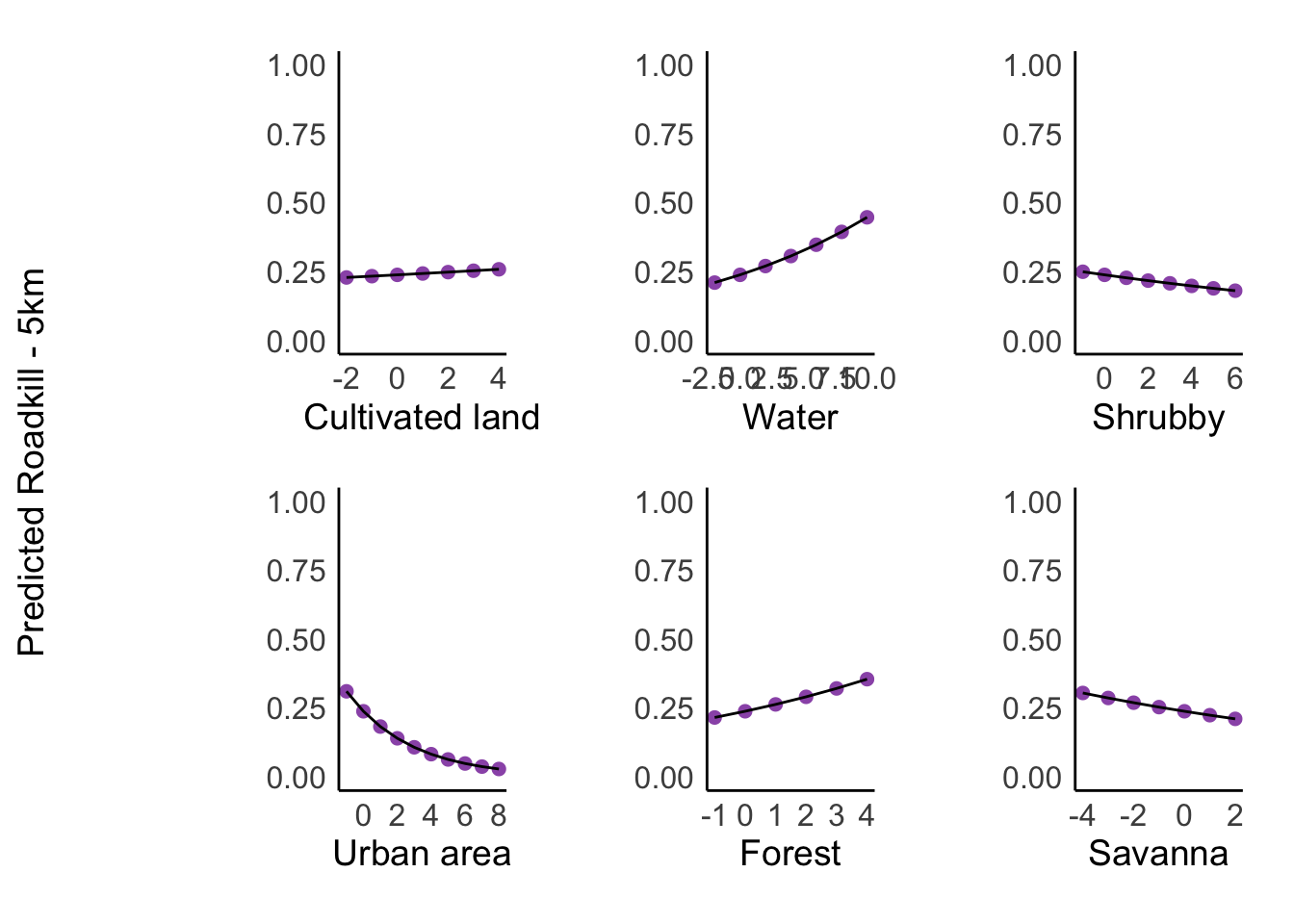

Preliminary conclusions

The model outputs indicate that paved roads significantly increase wildlife roadkill rates, as does traffic volume, supporting our initial hypotheses. However, contrary to expectations, pavement type did not differentially affect roadkill rates across taxonomic groups (reptiles, birds, mammals) in the current dataset.

Seasonality emerged as another critical factor. In this region of Brazil, the rainy season coincides with higher temperatures, which aligns with peak activity periods for most local species, likely explaining the elevated roadkill records during this time.

Forest cover became a significant driver of roadkill at larger scales (3–5 km), supporting our hypothesis that broader spatial extents better capture habitat availability. These areas likely act as connectivity corridors, shaping animal movement patterns and increasing collision risks near roads.